␥ Fiber Bundles

A fiber bundle is a sequence of maps of the form

where $\mathcal F$ is the fiber, $\mathcal E$ is the total space, and $\mathcal M$ is the base space. As the notation suggests, $\iota$ is an injective map referred to as the inclusion which “places” the fiber $\mathcal F$ vertically inside $\mathcal E$. Meanwhile, $\pi$ is a surjective map known as the projection — given a point $q\in\mathcal E$, the point $\pi(q)\in\mathcal M$ is the shadow cast by $q$ down on the base space.

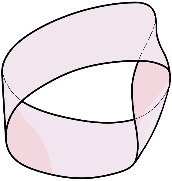
The preimage under $\pi$ of the point $p\in\mathcal M$ is diffeomorphic to $\mathcal F$, and is called “the fiber above $p$”. The job of $\iota$ is to tell us what “a typical fiber” in $\mathcal E$ looks like. The typical fiber of the Hopf fibration is a circle:

A principal $G$-bundle is one whose fiber $\mathcal F = G$ is a Lie group, and where each fiber has a right $G$-action that is compatible with the fiber bundle structure in a certain way. The reason why we consider a right action is that we can create principal bundles out of homogeneous spaces , and in doing so, the right-action on the fiber must play nice with the left-action of the homogeneous space. Let’s assume you know a bit about homogeneous spaces, and begin our story there.

␥ Coset Spaces

A homogeneous space refers to a smooth manifold $\mathcal M$ equipped with a left $G$-action (satisfying some axioms). We let $g\in G$ act on $p\in\mathcal M$ to yield $g\cdot p\in \mathcal M$. A homogeneous space does not have a distinguished point (think of a sphere, on which no point is more special than the other). However, if we do choose a special point $p_0\in\mathcal M$ (sort of like choosing the origin of a coordinate system), we can view $\mathcal M$ as a coset space . We do so by considering the subgroup $G_{p_0} < G$ of group actions that leave the point $p_0$ fixed — the stabilizer subgroup of $p_0$ in $G$. Denoting the subgroup $G_{p_0}$ as $H$, we have the following picture:

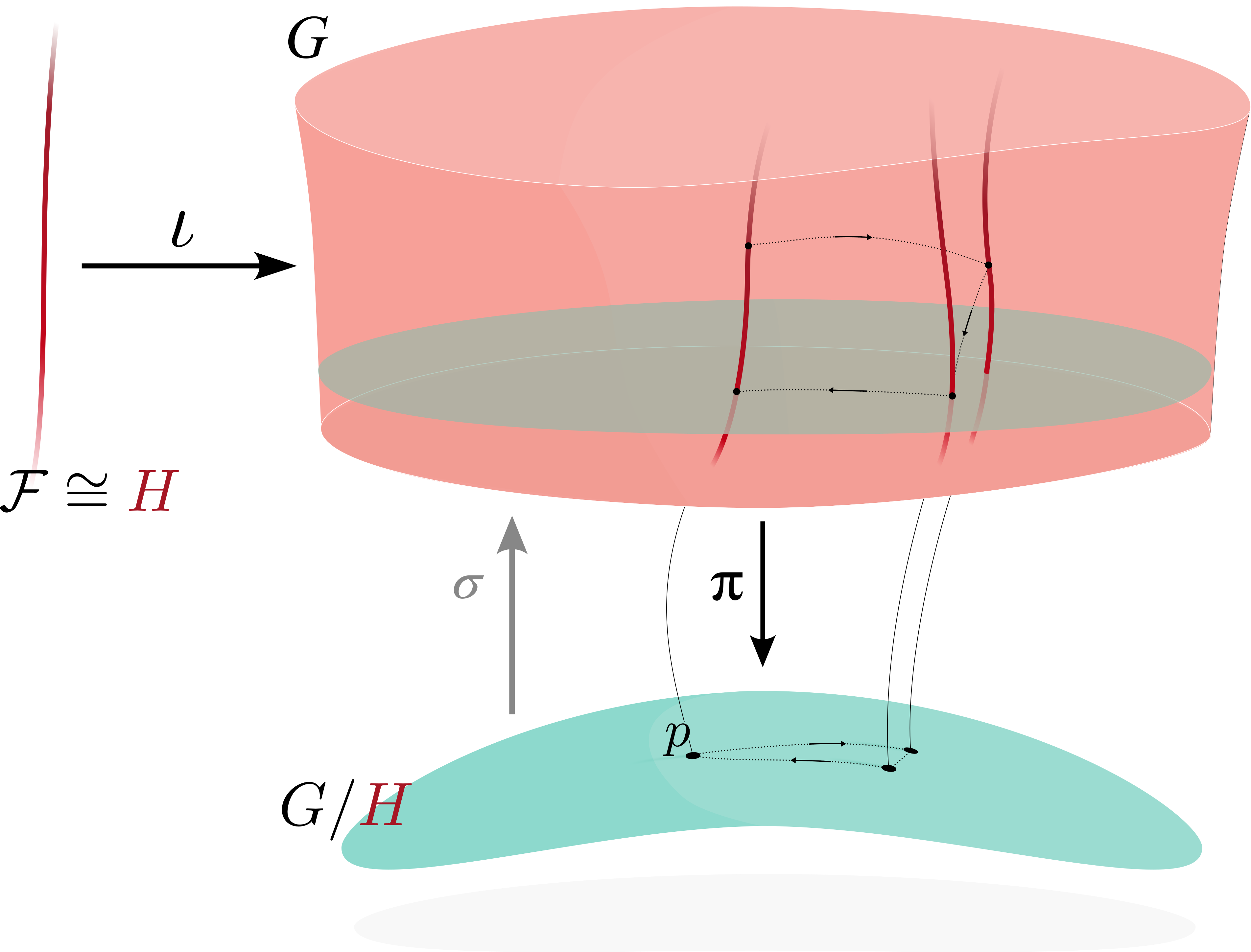
which is that of a principal $H$-bundle. The map $\pi$ sends $g\in G$ to the point $g \cdot p_0$, and we observe that $\pi(g)=\pi(gh)$ for any $g\in G$ and $h\in H$. We define a section (think cross-section) of this bundle to be a map $\sigma$ that is a right-inverse of $\pi$, i.e., $\pi \circ \sigma=\mathrm{id}_{G/H}$ is the identity map on $G/H$.¹

Example 1 (Spheres). $SO(3)$ acts on the sphere $S^2$. Given a point $p\in S^2$, the rotations about the axis passing through $-p$ and $p$ are the stabilizer subgroup $SO(3)_p$. Then, $SO(3)/SO(3)_p$ is isomorphic to $S^2$, and we get a fiber bundle

Observe that $SO(3)_p\cong SO(2)$. Due to this isomorphism, you will often see the claim $SO(3)/SO(2) \cong S^2$. However, it is important to note that there is no unique map $SO(2) \overset{\iota}{\rightarrow} SO(3)$ (any one-parameter subgroup of $SO(3)$ is isomorphic to $SO(2)$)!

Example 2 (Hopf Fibration). The set of unit quaternions² $\mathbb Q_S$ can be identified with the matrix Lie group $SU(2)$. Quaternions act on points in $\mathbb R^3$ via rotations, with the quaternions $q,-q$ representing the same rotation. Suppose $H\leq SU(2)$ is all the rotations about a fixed axis, let’s say the rotations about the $\mathrm{z}$-axis. The resulting bundle $H\hookrightarrow SU(2) \rightarrow S^2$ is what is visualized in the video above (also see the appendix)! Note that $H\cong SO(2)\cong S^1$.

Example 3 (SPD Matrices). Let the set of $n\times n$ symmetric positive-definite matrices be written as $\mathrm{SPD}(n)$. Given a matrix $g\in GL(n)$, it acts on $\boldsymbol\Sigma\in\mathrm{SPD}(n)$ as $\boldsymbol\Sigma \mapsto \mathbf g\boldsymbol\Sigma \mathbf g^\top$, where $g\mapsto \mathbf g$ is the standard representation of $GL(n)$ as $n\times n$ matrices. To see the coset space structure of $\mathrm{SPD}(n)$, we need to choose a distinguished point on it, and the fiber sitting above it will be the group of elements that leave the distinguished point fixed. I leave this as an exercise, with a hint in the footnotes!³

Conversely, given a Lie group $G$ and a subgroup $H\leq G$, we can view $G/H$ as a homogeneous space. A point in $G/H$ is of the form $gH$. The fiber sitting above $gH$ may also be denoted as $gH$, but technically refers to the subset

a left coset of $H$ in $G$. The map $\pi$ projects $g$ to its coset $gH\in G/H$ (as explained in one of my earlier posts ), with the identity coset $eH$ viewed as being a distinguished point on $G/H$. Importantly, we also have a right $H$-action on the group. This right-action preserves fibers, since for every $gh_1\in gH$ and $h_2\in H$, we have $(gh_1)h_2 \in gH.$ Thus, given a subgroup $H < G$ we not only get a homogeneous space $G/H$, but we can also endow $G$ with the structure of a principal $H$-bundle. The homogeneous space structure lets us move “horizontally” in $G$ using the left $G$-action, while the principal bundle structure lets us move “vertically” using the right $H$-action. The following examples are the two extreme cases where we can only move horizontally or vertically. In Example 4, the fiber is trivial, and all of the content of the total space $G$ is in the base space — vice versa for Example 5.

Example 4 ($G$-Torsor). This is the principal $\lbrace e\rbrace$-bundle where $G$ sits “horizontally”, defined by $e\hookrightarrow G \rightarrow G/\lbrace e \rbrace$. When $G=(\mathbb R^n, +)$ (where the group operation is vector addition) and $e=\mathbf 0$ (the zero vector of $\mathbb R^n$), the principal $\mathbb R^n$-torsor we constructed above is the $n$-dimensional affine space (without the scalar multiplication operation). In other words, this is $\mathbb R^n$ with the origin “forgotten”.

Example 5 (Principal $G$-Bundle over a Point). This is the fiber bundle where $G$ sits “vertically” over a single point, defined by $G\hookrightarrow G \rightarrow \lbrace 🐈 \rbrace$. We can replace 🐈 by any other object, doesn’t matter.

Principal Bundles

In the above, we constructed the fiber bundle $H\hookrightarrow G \rightarrow G/H$. We showed that we can then view $G/H$ as being a homogeneous space with a left $G$-action, and $G$ as a principal $H$-bundle with a right $H$-action that preserves fibers. Turns out that these objects carry too much information, and we need to discard some of this information to narrow our focus. For instance, $G/H$ is technically only a homogeneous space after we stop viewing the identity coset $eH$ as being a special point. As Example 4 shows, every Lie group can itself be viewed as a homogeneous space once we “forget” the identity element. Similarly, a general principal $H$-bundle may not come with a left $G$-action, as exemplified in the next section.

Example 6 (Tangent Bundle). Let $\mathcal M$ be a smooth $n$-dimensional manifold. The tangent space at a point $p\in \mathcal M$ is denoted as $T_p\mathcal M$, and the union of these tangent spaces is written as $T\mathcal M$. We can define a unique smooth structure on $T\mathcal M$ that makes the following maps smooth:

This fiber bundle has a fiber-preserving $GL(n)$ action — matrix-vector multiplication. However, $T\mathcal M$ is not a principal $GL(n)$-bundle since its fibers are not isomorphic to $GL(n)$. Nevertheless, there is indeed a principal $GL(n)$-bundle closely related to $T\mathcal M$, which is…

␥ The Frame Bundle

Consider an ordered set of $n$ linearly independent vectors in $T_p\mathcal M$. One such set is called a frame. The space of all the frames at $p$ make up the fiber, and the union of these fibers leads to the notion of a frame bundle $F\mathcal M$. More formally, we can view a frame at $p\in\mathcal M$ as being a linear isomorphism from $\mathbb R^n$ to $T_p\mathcal M$. The frame bundle is then (as a set) the following object:

The frame bundle has an action of $GL(n)$. We need to take care that this is a right-action and not a left-action, the difference being that the group element $gh \in GL(n)$ should act on a vector $(p,v)\in T\mathcal M$ as

On the other hand, a left-action of $gh$ would look different — $h$ will act first, then $g$.

This is where the linear-isomorphisms interpretation of the frame bundle comes in handy; given an $n\times n$ matrix $\mathbf A\in GL(n)$, we let

where $[f\circ \mathbf A](\mathbf v) = f(\mathbf A \mathbf v)$. There is a way to view $T\mathcal M$ as a fiber bundle that is “ associated ” to the frame bundle. We say that $GL(n)$ is the structure group of $T\mathcal M$, and we call $T\mathcal M$ a $GL(n)$-bundle. An associated bundle has a left action of its structure group. If that is confusing as hell, then you’re on the right track.

␥ Ehresmann Connections

Think of the fibers as trees in a forest. Consider the plight of our monkey, Ehresmann . It is clear to him how to climb up and down a tree (using the right $H$-action), but Ehresmann wants to jump from one tree to another. He needs to decide what constitutes horizontal movement! Will he jump such that his height off the ground is the same before and after the jump? Will he jump so that the tree length $\ell$ (as measured from the ground) is the same? Perhaps he will jump in a direction perpendicular to his tree?

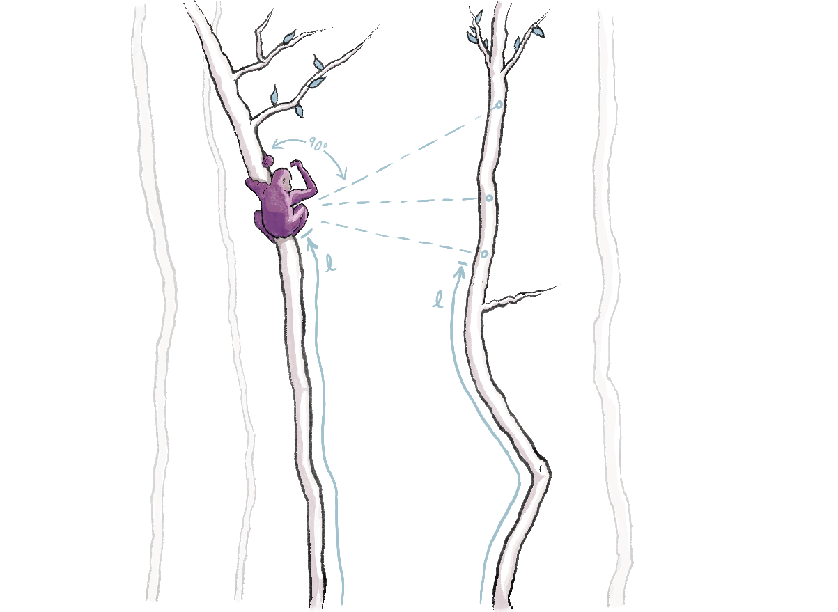
Assume Ehresmann the monkey is at the point $q \in \mathcal E$. The space of all the directions in which he could jump constitute the tangent space, $T_{q}\mathcal E$. The vertical subspace $\text{Ver}_q\mathcal E$ is all the directions that keep Ehresmann on the same tree. It is precisely the vectors $v$ that satisfy $d\pi_q(v)=0$; these directions do not change Ehresmann’s coordinates as measured along the ground. The vertical subspaces, collectively called the vertical subbundle $\text{Ver}\mathcal E$, are well-defined as soon as we define a principal bundle.

The horizontal subbundle is something that must be chosen, similar to how we choose an inner product on a vector space. Turns out that there are a few different, equivalent ways of specify a horzontal subbundle for a principal $H$-bundle:

1. specify a horizontal subspace $\text{Hor}_q\mathcal E \subseteq T_{q}\mathcal E$ for each $q\in\mathcal E$ such that $$T_q\mathcal E =\text{Hor}_q\mathcal E\oplus \text{Ver}_q\mathcal E,$$
2. choose a linear projection $\Gamma:T\mathcal E \rightarrow \text{Ver}\mathcal E$ and define $\text{Hor}\mathcal E \coloneq \mathrm{ker}(\Gamma)$,⁴
3. write down a $T\mathcal E$-valued one-form $\Gamma$ on $\mathcal E$ that satisfies $\Gamma\vert_{\text{Ver}\mathcal E}=\mathrm{id}_{\text{Ver}\mathcal E}$ (i.e., $\Gamma$ restricted to $\text{Ver}\mathcal E$ is the identity map on $\text{Ver}\mathcal E$), or
4. write down an $\mathfrak h$-valued one-form $\Gamma$ on $\mathcal E$.

It takes some self-introspection and a few dozen cups of coffee to see why these are indeed equivalent objects (i.e., neither of them specifies too much or too little structure!). An Ehresmann connection is a choice of horizontal subbundle that satisfies a few additional properties (cf. Sec. 10.1), most notably the $H$-invariance condition:

where $R_g:\mathcal E \rightarrow \mathcal E$ is the right-action of $g\in H$ on $\mathcal E$, and $(R_g)_*$ is the corresponding pushforward map on tangent spaces. This condition ensures that the right $H$-action on $\mathcal E$ preserves all the horizontal subspaces. Note that we can write an analogous condition for $\text{Ver}\mathcal E$, but since the vertical subbundle does not depend on a choice of connection, it is automatically satisfied!

The $H$-invariance condition can also be written in terms of the connection form:

␥ The Maurer-Cartan Form

When we used a coset space to create a principal $H$-bundle, we used the sequence of smooth maps $H\hookrightarrow G \rightarrow G/H.$ This gives us a corresponding sequence of linear maps:

which is a short exact sequence in the category of vector spaces. Here, $\mathfrak g/\mathfrak h$ does not necessarily have a canonically defined Lie bracket for the same reason that $G/H$ is not necessarily a Lie group. Furthermore, there is generally no canonical way of viewing the quotient vector space $\mathfrak g/\mathfrak h$ as a subspace of $\mathfrak g$ — this is a choice that must be made. It is precisely the choice that is made by an Ehresmann connection.

But that is not the topic of this section… in this section, we will consider the “completely vertical” bundle $G\hookrightarrow G \rightarrow \lbrace 🐈 \rbrace$ from Example 5. This is the principal $G$-bundle that has a single fiber sitting above 🐈. You might say that there is no choice of horizontal subspace to be made here, since $TG=VG$. But there is indeed a choice of horizontal subspace, it just happens to be the trivial choice of $HG=\lbrace \mathbf 0 \rbrace$. Since there is exactly one Ehresmann connection on this bundle, and given the various equivalent ways of defining a connection, what is the corresponding $\mathfrak g$-valued one-form?

Given a vector $X\in\mathfrak g$, we can drop a vector field $\widetilde X$ on $G$ using its right-action on itself:

This happens to be the left-invariant vector field (LIVF) of $X$. The Ehresmann connection is then the map $\omega:TG \rightarrow \mathfrak g$ that sends $\widetilde X$ to $X$:

and is called the Maurer-Cartan form of $G$. Observe that $\omega_g=L_{g^{-1}*}$. It is an exercise for the reader to verify that the Maurer-Cartan form satisfies the $G$-invariance condition

for all $g\in G$.⁵ The uniqueness of the Maurer-Cartan form (as an Ehresmann connection on the Example 5 bundle) is shown in Theorem 10.3 of Sontz . At the 22 minute mark , Schuller shows a connection between $\omega$ and local representations of connections.

The exterior derivative of an Ehresmann connection is related to the curvature of the horizontal subbundle; I characterize the exterior derivative of $\omega$ in Appendix B.

␥ The Christoffel Symbols

What we call “a connection” in differential geometry can be viewed as an Ehresmann connection on the frame bundle. Given a coordinate chart $(U, x^i)$ on $\mathcal M$, we get a local section $\sigma$ of $F\mathcal M$ over $U$, defined by

Given a connection form $\boldsymbol\Gamma$ on $F\mathcal M$, we can pull it back under $\sigma$ to get $\boldsymbol{\overline\Gamma}\coloneq \sigma^\ast \boldsymbol\Gamma$. We can then express it in the coordinate frame as $\boldsymbol{\overline\Gamma}=(\boldsymbol{\overline\Gamma})_{i}dx^i$. But ${\overline\Gamma}$ takes values in $\mathfrak {gl}(n)$, which means that we can write $\boldsymbol{\overline\Gamma} = {{\overline\Gamma}}^m_{ni}dx^i$. The coefficients ${{\overline\Gamma}}^m_{ni}$ are precisely the Christoffel symbols of the connection in the coordinate chart $(U,x^i)$. This formulation of the Christoffel symbols shows why they are not tensorial quantities; the $m$ and $n$ indices correspond to the $\mathfrak{gl}(n)$-valued nature of the connection form, while the $i$ index is tensorial.

A choice of horizontal subbundle lets us parallel transport vectors along curves on $\mathcal M$. Given a curve $\gamma:[0,1]\rightarrow \mathcal M$ and a frame $e\in F_{\gamma(0)}\mathcal M$, we can lift $\gamma$ to a curve $\widetilde \gamma:[0,1]\rightarrow F\mathcal M$ such that $\pi \circ \widetilde\gamma = \gamma$, $\widetilde\gamma(0)=e$, and $\widetilde\gamma'(t) \in \text{Hor}_{\widetilde\gamma(t)}F\mathcal M$ for all $t\in[0,1]$. This is called the horizontal lift of $\gamma$ starting at $e$. The frame at $\widetilde\gamma(1)$ is then the parallel transport of the frame at $\widetilde\gamma(0)$ along $\gamma$. The illustration at the top of this post also explains holonomy: the observation that parallel transporting a vector along a loop may not return the vector to its original position.

Appendix A. Visualizing the Hopf Fibration

Here are some functions in Julia that I used to animate the Hopf fibration:

 1
 2
 3
 4
 5
 6
 7
 8
 9
10
11
12
13
14
15
16
17
18
19
20
21
22

# section σ:S²→S³
function σ(p₁,p₂,p₃)
    1/sqrt(2*(1+p₃)) * quat(1 + p₃, -p₂, p₁, 0)
end

# stabilizer subgroup of (0,0,1)
H = [quat(cos(angle), 0, 0, sin(angle)) for angle in range(0, 2π, 1000)]

# preimage of {p} under π:S³→S²
function π⁻¹(p)
    p₁,p₂,p₃ = p
    f_quat = σ(p₁,p₂,p₃) .* H
    map(f_quat) do q
        r = real(q)
        (acos(r)/(π * sqrt(1-r^2)) .* imag_part(q) .+ (0, 0, 1.6)) .* 1.5
    end
end

# parametrization of the sphere Ψ:ℝ²→S³
function sphere(ϕ,θ)
    (sin(ϕ)*cos(θ), sin(ϕ)*sin(θ), cos(ϕ))
end

Appendix B. Maurer-Cartan Structure Equation

Given a basis $(E_i)_{i=1}^n$ for $\mathfrak g$, the Maurer-Cartan form can be expressed as

which eats a vector field and returns a function from $G$ to $\mathfrak g$, i.e., $\omega:\mathfrak X(TG)\rightarrow C^\infty(G,\mathfrak g)$. Some of its properties are:

• It is left-invariant since its components in the left-invariant coframe are constants (rather than functions).
• If it eats a LIVF, then the resulting function is a constant: $\omega(\widetilde X)=X^i E_i=X$.
• An arbitrary vector field can be written as $f^i\widetilde E_i$, where $f^i:G\rightarrow \mathbb R$ need not be constant. We have, $\omega(f^i\widetilde E_i)=f^i\omega(\widetilde E_i)=f^i E_i.$

Basically, $\omega$ trivializes the tangent bundle $TG$ into $G\times \mathfrak g$. The exterior derivative of $\omega$ is defined via the formula in Prop. 14.29 of Lee ISM :

Because $\varepsilon^i(\widetilde X)$ and $\varepsilon^i(\widetilde Y)$ are constant, we have

where $c_{jk}^i$ are the structure constants of $\mathfrak g$ in the basis $(E_i)_{i=1}^n$. This equation is called the Maurer-Cartan structure equation. For any two $\mathfrak g$-valued forms, we can define

Setting $\eta=\omega$, we get

Hence, we can write $d\omega=-\frac{1}{2}\omega\wedge \omega=-\frac{1}{2}E_ic^i_{jk}\varepsilon^j\wedge \varepsilon^k$.⁶

Suppose we choose a matrix representation $\boldsymbol\Phi:G\rightarrow GL(m,\mathbb R)$. Then, $d\boldsymbol\Phi_e$ is a representation of $\mathfrak g$. Let $\boldsymbol\omega\coloneqq d\boldsymbol\Phi_e\circ\omega$ be a $\mathfrak{gl}(m)$-valued one-form on $G$. We have,

Finally, we will choose a parametrization $\psi:\mathbb R^n\rightarrow G$ and pull back $\boldsymbol\omega$ and $d\boldsymbol\omega$ under $\psi$. First, we do this for $\boldsymbol\omega$:

Let $\psi^\ast\varepsilon^i=\epsilon_{i}dx^i$. Then

in the notation of my previous post . Hence,

which is a $d\boldsymbol\Phi_e(\mathfrak{g})$-valued one-form on the parameter space $\mathbb R^n$, where $\boldsymbol\psi\coloneqq\boldsymbol\Phi \circ \psi$.

Let $\boldsymbol\omega^\vee \coloneqq (\,\cdot\,)^\vee\circ d\boldsymbol\Phi_e\circ\omega$. Then, we have $\psi^\ast \boldsymbol\omega^\vee(\mf y)=J(\mf x)\mf y$ for all $\mf y\in T_{\mf x}\mathbb R^n$, or in terms of components, $\psi^\ast \boldsymbol\omega^\vee=\mf J_jdx^j$, where $\mf J_j$ is the $j^{th}$ column of $\mf J$.

Pullbacks commute with the exterior derivative and linear transformations, which simplifies the pullback of $d\boldsymbol\omega$:

On the other hand, we can also move $d$ ‘inwards’ past the linear operators:

Hence,