The Lie Group-Lie Algebra Correspondence

A topological group is a set of elements $G$ that has both a group operation $\odot$ and a topology . The group operation satisfies the usual axioms (same as those of finite groups ), and the presence of a topology lets us say things like ’the group is connected’ and ’the group operation is continuous’. $G$ is called a Lie group if it is also a smooth manifold. The smooth structure of the manifold must be compatible with the group operation in the following sense: $\odot$ is differentiable with respect to either of its arguments ¹. The compatibility of its constituent structures is what makes a Lie group so special, enabling it to capture the essence of a continuous symmetry .

A different (but closely related) mathematical object is the Lie algebra. A Lie algebra $\mathfrak v$ is a vector space equipped with an operation called the Lie bracket, $[\cdot, \cdot]: \mathfrak v \times \mathfrak v \to \mathfrak v$, that satisfies certain properties that parallel those of a ‘cross product’. While a Lie algebra may exist in the absence of an associated Lie group, every Lie group gives rise to a Lie algebra². In other words, we can associate to each Lie group $G$ a corresponding Lie algebra, with the latter typically denoted as $\mathfrak g$ to emphasize its relationship to $G$.

Letting $e$ denote the identity element of $G$, we will see that $T_e G$ (the tangent space of $G$ at $e$), together with an appropriately defined bracket operation, is a natural candidate for $\mathfrak g$. Consider as an example $SO(2)$, the group of rotation matrices of $\mathbb R^2$ having determinant $1$, whose identity element $e$ is the identity matrix $I$. The tangent space $T_ISO(2)$ consists of the $2\times 2$ skew-symmetric matrices. Skew-symmetric matrices represent infinitesimally small rotations, since near the identity element of $SO(2)$ (i.e., the identity matrix), we have

$$\begin{align} \theta \approx 0 \Rightarrow \begin{bmatrix} \ \ \cos\theta & -\sin\theta\ \ \\ \ \ \sin\theta & \cos\theta \end{bmatrix} \approx I + \begin{bmatrix} \ 0 & -\theta \ \\ \ \theta & 0 \end{bmatrix} \end{align}$$

Still, the above observation alone does not make it clear what the relationship between $SO(2)$ and $T_ISO(2)$ is. For starters, why should one expect infinitesimal rotations to be related in any way to arbitrary (large angle) rotations? What is the significance of the Lie bracket?

This post is by no means meant to be an introduction to Lie groups; for that, I recommend the first few chapters of Brian C. Hall’s book. I will instead hurry us along to our main line of investigation – understanding the Lie group-Lie algebra correspondence, pausing only to show you some pictures/diagrams that I had fun drawing. A bonus takeaway from this post will be a deeper understanding of the exponential map, one that unifies the exponentials of real numbers, complex numbers, and matrices.

---

Background

The details in this section may be skipped , but I suggest looking at the illustration below before moving on.

Pushforwards

Given a smooth, parameterized curve $\gamma:\mathbb R \rightarrow G$, let $(U,h)$ be a chart of $G$ such that $\gamma (0)\in U$. Observe that $h\circ \gamma:\mathbb R\rightarrow \mathbb R^n$ can be differentiated in the usual way, and that $\frac{d}{dt}\left[h\circ \gamma (t)\right]\big\vert_{t=0}$ is simply a vector in $\mathbb R^n$. All of the curves on $G$ that result in a given vector of $\mathbb R^n$ when differentiated as above represent the same tangent vector, i.e., a single element of the tangent space $T_{\gamma(0)}G$.

Let $[$$\gamma$$]$ denote the tangent vector (or more precisely, the equivalence class) corresponding to the curve $\gamma$. We say that $[$$h\circ \gamma$$]$ is the pushforward of the tangent vector $[$$\gamma$$]$ under the map $h$. More generally, if $f:\mathcal M \rightarrow \mathcal N$ is a smooth map between manifolds, then the differential of $f$ at $p\in \mathcal M$ is the linear operator that maps tangent vectors at $p$ to their pushforwards at $f (p)$:³

$$\begin{align} (f_*)_p:\ T_p \mathcal M &\rightarrow T_{f (p)} \mathcal N\\ \mathbf v &\mapsto (f_*)_p \mathbf v \nonumber \end{align}$$

In practice, $(f_*)_p$ ends up looking something like the Jacobian of $f$ evaluated at $p$. The caveat is that a Jacobian (matrix) maps vectors in $\mathbb R^n$ to vectors in $\mathbb R^m$, whereas $(f_*)_p$ does the more general job of mapping vectors in $T_p \mathcal M$ to vectors in $T_{f (p)} \mathcal N$.

Given $g\in G$, let $\mathcal L_g:G\rightarrow G$ denote left-multiplication by $g$, i.e., $\mathcal L_g(h) = g\odot h$ for all $h\in G$. Here’s how a tangent vector at the identity $e\in G$ can be ‘pushed forward’ by the left-multiplication map $\mathcal L_g$:

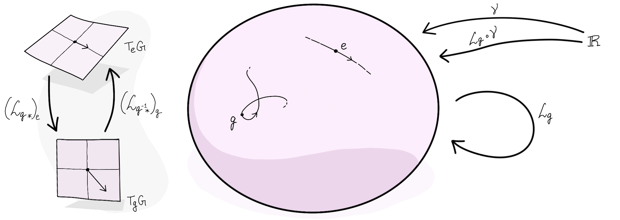
where the curve passing through $g$ was obtained by composing $\gamma$ with $\mathcal L_g$. Since $T_eG$ is going to be identified⁴ with $\mathfrak g$ (as a vector space), the above illustration is going to play a key role in the forthcoming discussion. It shows that $(\mathcal L_{g^{-1}*})_g$$=(\mathcal L_{g*})_e ^{-1}$ will reduce a tangent vector at $g$ to an element of the Lie algebra.

By reuse of notation, we can also ‘push forward’ entire vector fields (when $f$ is a diffeomorphism):

$$\begin{align} f_*:\ \mathfrak X (\mathcal M) &\rightarrow \mathfrak X (\mathcal N)\\ X &\mapsto f_* X \nonumber \end{align}$$

where $\mathfrak X(\cdot)$ denotes the set of all smooth vector fields on a manifold.

Morphisms

Most (if not all) mathematical objects come with a distinctive structure; for topological spaces, it is their topology/open sets, for vector spaces their vector addition and scalar multiplication operations, for finite groups the existence of inverses, and so on. Mappings between objects of the same type that preserve these structures are called homomorphisms (or in the jargon of category theory, simply morphisms). The homomorphisms between vector spaces are the linear transformations between them. Suppose $f:V\rightarrow W$ is a linear transformation, then

$$f(v_1 \overset{V}{+}v_2)=f(v_1)\overset{W}{+}f(v_2) \in W,$$

which shows that the structure of the vector addition operation $\overset{V}{+}$ of $V$, has been transported to that of the $\overset{W}{+}$ operation of $W$. This suggests that homomorphisms (i.e., structure-preserving maps) may be paramount to the study of the underlying mathematical structure, which is indeed the case (see linear algebra).

If $A$ and $B$ are two objects of the same type and $f$ a homomorphism between them, we simply write

$$\begin{array}{c} A \overset{f}{\longrightarrow} B \end{array}$$

where the meaning of $f$ depends on which type of mathematical structure is being transported. A homomorphism for which there also exists an ‘inverse homomorphism’ $g:B \rightarrow A$, such that $f \circ g = g\circ f =\$the identity map, is called an isomorphism. Isomorphisms between vector spaces are those linear transformations that can be represented as invertible matrices. Beware that neither word, homomorphism or isomorphism, should be uttered unless the structure in question is contextually obvious. Two objects are never simply isomorphic, they are isomorphic as vector spaces, or isomorphic as topological spaces, and so on.

A homomorphism between topological spaces is a continuous map between them. The word homeomorphism, rather confusingly, refers to an isomorphism (and not a homomorphism) between topological spaces; this piece of nomenclature is quite a tragedy. An isomorphism between smooth manifolds is a differentiable map with a differentiable inverse – a diffeomorphism.

A Lie group homomorphism $\varphi$ is a map between two Lie groups that preserves both the group operation and the topology; i.e., it is simultaneously a group homomorphism and a continuous map. The best way to understand what a group homomorphism entails is through a commutative diagram:

We say that this diagram commutes if the two compositions of arrows (top-right and left-bottom, each of which results in $\searrow$) are in fact the same arrow:

$$\begin{align} \mathcal L_{\varphi (g)}\circ \varphi = \varphi \circ \mathcal L_g \end{align}$$

where $\circ$ indicates the composition of functions. Feeding an argument $\tilde g\in G$ on either side, we get

$$\begin{align} \varphi (g) \overset{H}{\odot}\varphi(\tilde g) &= \varphi (g \overset{G}{\odot} \tilde g) \\ \end{align}$$

where $\overset{G}{\odot}$ is the group operation in $G$ and $\overset{H}{\odot}$ is the group operation in $H$. This makes it (at least notationally) clear that $\varphi$ preserves the group structure, though one should work out the consequences of this definition; for instance, it can be shown that $\varphi$ should map the identity of $G$ to the identity of $H$. An example of a Lie group homomorphism is the determinant of a matrix, $\textrm {det}:GL(n;\mathbb R) \rightarrow \mathbb R^\times$, since

$$\begin{align} \textrm {det}(AB) = \textrm {det}(A) \textrm{det}(B) \end{align}$$

Here, $GL(n;\mathbb R)$ is the general linear group consisting of $n\times n$ invertible matrices and $\mathbb R^\times$ is the multiplicative group of real numbers (crucially, $0\notin \mathbb R^\times$). Observe that $\textrm {det}(I)=1$ as promised.

---

Invariant Vector Fields

As I hinted at previously, the key to uncovering the Lie group-Lie algebra correspondence is to study the topological and group structures of $G$ simultaneously. How does one do this? A good starting point would be to specialize the curves and vector fields considered above (which are topological objects) to those special ones that also respect the group structure of $G$.

This brings us to a central object in the study of Lie groups, the space of left/right-invariant vector fields. A left-invariant vector field is one for which the vectors at two different points are related by the pushforward operator $\mathcal L_{g*}$ corresponding to left-multiplication by the group elements. More rigorously, a vector field $X\in \mathfrak X (G)$ is said to be left-invariant if the following diagram commutes:

For example, we have for $h\in G$,

$$\begin{align} X \circ \mathcal L_g (h) = (\mathcal L_{g*})_h X(h) \end{align}$$

$=X(g\odot h)$. An important consequence of this definition is that just by knowing $X(e) \in T_e G$, we can determine the value of $X$ at all the other points, since $X(g) = (\mathcal L_{g*})_e X(e)$. In fact, one can construct a left-invariant vector field by picking any vector $\tilde X \in T_eG$ and defining $X(g) \coloneqq (\mathcal L_{g*})_e \tilde X$. Conversely, given a left-invariant vector field $X$, we can simply evaluate it at the identity $e$ to determine the $\tilde X$ that generated it. Thus, the space of left-invariant vector fields on $G$, written as $\mathfrak X^{\mathcal L}(G)$, is isomorphic to $T_eG$ as a vector space (the fact that $\mathfrak X^{\mathcal L}(G)$ can be given a vector space structure is for the reader to deduce). The word ’left-invariant’ comes from the fact that $\mathcal L_{g*}X= X$.

A left-invariant vector field $X\in \mathfrak X^{\mathcal L}(G)$ is special because it represents ‘water’ flowing along the surface of $G$ in perfect concordance with the group structure of $G$. The fact that such an object can be related to $T_eG$ bodes well for the establishment of $T_eG$ as an object that corresponds to the Lie group $G$. However, some reflection will show that we need to do more work to recover the group structure of $G$ at $T_eG$. For starters, the group multiplication operation $\odot$ need not be commutative, whereas the vector addition operation $+$ in $T_eG$ is commutative by definition. This is where the Lie bracket comes in; it is a multiplication-like operation that can be imposed on $T_e G$ to in some sense ‘measure the failure of commutativity’ in $G$. We will revisit this point a little later.

The Exponential Map

If the Lie algebra is to correspond to the Lie group, the elements of the Lie algebra should be somehow associated with the elements of the Lie group. How do we associate $\tilde X \in T_eG$ to a unique group element of $G$? First, we extend $\tilde X$ to the unique left-invariant vector field $X$ that satisfies $X(g) = (\mathcal L_{g*})_e \tilde X$. Thereafter – and this is going to sound silly – we place a ‘boat’ at the identity $e$ and let it flow along the surface of $G$ in the direction of $X$ for exactly one unit of time!

Let’s unpack what that means. The boat is going to trace out a path/curve on $G$, which we denote by $\gamma :[0, 1] \rightarrow G$, such that $\gamma (0)=e$. At time $t\in[0,1]$, the boat’s position is given by $\gamma(t)\in G$. Its velocity at time $t$ is given by $\gamma ^\prime(t)=X(\gamma(t))$. Thus, we require that

$$\begin{align} \gamma ^\prime(t) = \big(\mathcal L_{\gamma(t)*}\big)_e \tilde X \end{align}$$

The equation above is a differential equation (or dynamical system) that can be solved to yield a solution (or trajectory) $\gamma (t)$. The solution is called an integral curve or a flow of $X$ starting at $e$. Of course, we can solve it by using the local charts of $G$ to (locally) reduce it to a system of ordinary differential equations in $\mathbb R^n$, and then ‘stitching’ the local solutions together to get the overall curve on $G$. Before I convince you that this can indeed be done, let’s exercise prescience in making the following definition :

$$\begin{align} \exp:\ T_e G &\rightarrow G\\ \tilde X &\mapsto \gamma(1) \nonumber \end{align}$$

where $\gamma$ is the integral curve (or flow) that solves $(8)$ for the given choice of $\tilde X$. Note that $\gamma ^\prime(0) = \tilde X$ is the initial velocity of the boat.

Example 1: $G=\mathbb R^\times$, the Multiplicative Group of Real Numbers

In this case, $\mathcal L_g$ and $(\mathcal L_{g*})_e$ reduce to the same operation – multiplication of real numbers⁵. Equation $(8)$ reduces to

$$\begin{align} \gamma ^\prime(t) = \gamma(t) \tilde X \end{align}$$

where $\tilde X \in T_e\mathbb R^\times \cong \mathbb R$ and $e=1$ is the identity element (of multiplication). By seeking a power series solution (or better yet, through an informed guess), we get

$$\begin{align} \gamma(t) = 1 + t\tilde X + \frac{t^2}{2!}\tilde X^2 + \frac{t^3}{3!}\tilde X^3 + \cdots \end{align}$$

so that $\exp(\tilde X)=\gamma(1)$ is the usual exponential function that we’ve come to know and love. By the uniqueness of the solution to an ODE, we have arrived at a well-defined definition for the exponential map in this case.

Example 2: $G=U(1) \cong SO(2)$, the Circle Group

$U(1)$ is the group of complex numbers of unit modulus, with the group operation $\odot$ being the multiplication of complex numbers. Since we have already seen how $(8)$ can be solved, a visual depiction of the exponential map might be more gratifying:

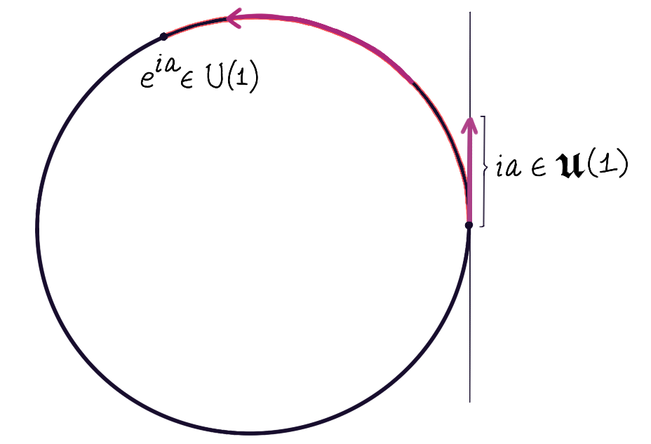
Because we are able to visualize this Lie group as a (topological) subspace of $\mathbb R^2$, we can quite literally see the boat flowing along the surface of $G$ in the direction of $X$. Here, $X(e^{i\theta})=e^{i\theta}\tilde X$, so the left-invariant vector fields are generated by sliding $\tilde X$ along the circle without changing its length.

Example 3: $G=GL(n;\mathbb R)$, the Invertible Matrices

Equation $(8)$ becomes

$$\begin{align} \gamma ^\prime(t) = \gamma(t) \tilde X \end{align}$$

(Just like in $\mathbb R^\times$, matrix multiplication and its differential both reduce to the same operation ⁵.) The rest follows in the same way as in Example 1.

Going back to Example 1, notice that a large negative initial velocity at $1\in \mathbb R^\times$ sends the boat to a small positive number, but never to $0$. For an analogous reason, $\exp(\tilde X)$ is always an invertible matrix. As the determinant of $\gamma(t)$ should change smoothly during the boat’s trajectory (and apparently it never hits the value $0$), we conclude that $\det(\exp(\tilde X))>0$. Thus, $\exp$ is once again not surjective.

Example 4: $G\cong \mathbb R$, the Shift Operators

The case for $G=\mathbb R$ with addition as the group operation seems rather uninteresting at first. Equation $(8)$ becomes

$$\begin{align} \gamma ^\prime(t) = \tilde X \end{align}$$

since the differential of the addition operation leaves the vector $\tilde X\in T_0 \mathbb R$ unchanged (after identifying all of the tangent spaces of $\mathbb R$ with $\mathbb R$). Thus, $\gamma(t)=t\tilde X + C$. Since $\gamma(0)=0$, we have $C=0$ and $\gamma(t)=t\tilde X$. This makes $\exp(\tilde X) = \gamma(1)=\tilde X$; the boat has moved away from the origin for $1$ unit of time under constant velocity. The same is true for $\mathbb R^n$, and in fact for any vector space with vector addition as the group operation.

The above result becomes interesting when we consider a group isomorphism from $\mathbb R$ to the space of shift operators . Consider an entirely new group $G$, and let $S^{a} \in G$ be something that operates on functions of the form $f:\mathbb R \rightarrow \mathbb R$ by shifting them to the left (if ${a} >0$) or right (if ${a}<0$) by ${a}$ units:

$$\begin{align} (S^{a} f)(t) = f(t + {a}) \end{align}$$

where ${a} \in \mathbb R$. Clearly, $e=S^0$ is the identity element of $G$ and $S^a\circ S^{-a} = S^0$. I defer the details to a footnote⁶, but a tangent vector in $T_{S^0}G$ is given by a differential operator of the form $\tau \frac{d}{dt}$, where $\tau \in \mathbb R$. The exponential map is then given by

$$\begin{align} \exp\left(\tau \frac{d}{dt}\right) = S^\tau \end{align}$$

It cannot be understated just how remarkable the above result is. Letting the left-hand side of $(15)$ operate on a function $f$ and evaluating the resulting function at $t_0$, we get

$$\begin{align} \left(\exp\left(\tau \frac{d}{dt}\right) f\right)(t_0) &= \left[\left( 1 + \tau \frac{d}{dt} + \frac{\tau^2}{2!} \frac{d^2}{dt^2} + \cdots \right) f\right](t_0) \end{align}$$

whereas on the right-hand side, we have $(S^\tau f )(t_0) =f(t_0+\tau)$. Thus,

$$\begin{align} f(t_0) + \tau \frac{df}{dt}(t_0) + \frac{\tau^2}{2!} \frac{d^2f}{dt^2}(t_0) + &\dots =f(t_0+\tau) \end{align}$$

which is nothing but the Taylor series expansion of $f$ at $t_0$! In a sense, the Taylor series expansion starts at $t_0$ and then ‘slides along the graph of $f$’ to obtain its value at the other points.

Properties of $\exp$

We have skipped a lot of the standard results in Lie theory in order to get to the fun parts of this blog post, but the following properties of $\exp$ are worth mentioning:

• It is always locally invertible near the identity element $0\in \mathfrak g$.
• Given a choice of $\tilde X\in \mathfrak g$, $\gamma(t)=\exp (t \tilde X)$ is a one-parameter subgroup of $G$, i.e., a Lie group homomorphism from $\mathbb R$ to $G$. Consequently, $\exp\big((t_1+t_2) \tilde X\big)=\exp(t_1\tilde X) \exp (t_2 \tilde X)$, and $\exp(-\tilde X)=\exp (\tilde X)^{-1}$.
• $\exp(t\tilde X)$ represent geodesic paths passing through the identity of $G$ with respect to a particular choice of metric (namely, a bi-invariant Riemannian metric, if one exists ) and the resulting Levi-Civita connection.

The Flows of $\mathfrak X^{\mathcal L}(G)$

Before we proceed, we need to see how the one-parameter subgroups $\exp(t\tilde X)$ can be extended to flows. A flow of $X\in \mathfrak X(G)$ is a map $\Phi:\mathbb R \times G \rightarrow G$ such that

$$\begin{align} \Phi(0,g) = g \quad \text{and} \quad \frac{d}{ds}\Big\vert_{s=t} \Phi(s,g) = X\big(\Phi(t,g)\big) \end{align}$$

Notice that $\Phi(\cdot , e ) = \gamma(\cdot)$ as before, but now we’re permitted to place the boat at any point $g\in G$ at $t=0$ and see how it flows. In this more general setting, the flow map $\Phi$ is given by

$$\begin{align} \Phi(t,g) = \mathcal R_{\gamma(t)}(g) \end{align}$$

where $\gamma(t) = \exp(t\tilde X)$. We say that flows of left-invariant vector fields are given by right-multiplications, and vice versa. As a function of $t$, $(19)$ is a trajectory that flows along the left-invariant vector field $X$ generated by $\tilde X$, passing through $g$ at $t=0$. Why is that? The velocity vectors along this trajectory are given by

$$\begin{align} \frac{d}{ds}\Big\vert_{s=t} \Phi(s,g) &= \frac{d}{ds}\Big\vert_{s=t} \mathcal R_{\gamma(s)}(g)\\ &= \frac{d}{ds}\Big\vert_{s=t} \big(g \odot \gamma(s)\big)\\ &= \frac{d}{ds}\Big\vert_{s=t} \mathcal L_g \gamma(s)\\ &= \big(\mathcal L_{g*}\big)_{\gamma(t)} \frac{d}{ds}\Big\vert_{s=t} \gamma(s)\\ \end{align}$$

Because $\gamma(t)$ solves $(8)$, we have

$$\begin{align} \frac{d}{ds}\Big\vert_{s=t} \Phi(s,g) &= \big(\mathcal L_{g*}\big)_{\gamma(t)} X\big(\gamma(t)\big)\quad \\ &= X\big(g \odot \gamma(t)\big)\\ &= X\big(\mathcal R_{\gamma(t)}(g)\big)\\ &= X\big(\Phi(t,g)\big). \end{align}$$

Lie Bracket

The fact that $\exp (t \tilde X)$ is a one-parameter subgroup of $G$ means that the corresponding subgroup must be Abelian, i.e., $\exp (t_1 \tilde X)$ and $\exp (t_2 \tilde X)$ commute under $\odot$ even if $\odot$ was not commutative in $G$. For instance, the (non-trivial) one-parameter subgroups of $SO(3)$ are rotations about a fixed axis – each of these is isomorphic to $SO(2)$, which is Abelian:

$$R_1,R_2\in SO(2) \Rightarrow R_1 \odot R_2 = R_2 \odot R_1$$

This means that we still haven’t captured the (potential) non-commutativity of the group at the Lie algebra. To do this, we first need to understand vector fields as derivations . An operator $X:C^\infty(G) \rightarrow C^\infty(G)$ is called a derivation if it is linear and satisfies the Leibniz rule:

$$X(f_1\cdot f_2) = f_1\cdot X(f_2) + f_2\cdot X(f_1)$$

with $f_1\cdot f_2$ indicating pointwise multiplication of $C^\infty(G)$ functions. Vector fields are derivations by construction , though we haven’t had to emphasize this aspect of them until now. When $X$ acts on a $C^\infty(G)$ function $f$, we will treat it as a derivation, but when $g \in G$, we will treat $X(g)$ as a tangent vector (which acts on one-forms instead).

For $X,Y\in \mathfrak X(G)$ and $f_1,f_2\in C^\infty(G)$, since $Y(f_1\cdot f_2)$ is again a $C^\infty(G)$ function, we can have $X$ act on it as follows:

$$\begin{align} X\big(Y(f_1\cdot f_2)\big) &= X\big(f_1\cdot Y(f_2) + f_2\cdot Y(f_1)\big)\\ &= f_1 \cdot X\big(Y(f_2)\big) + X(f_1)\cdot Y(f_2) \nonumber \\&\quad + f_2\cdot X\big(Y(f_1)\big) + X(f_2)\cdot Y(f_1)\\ \end{align}$$

which indicates that $X\big(Y(\ \cdot\ )\big)$ is not a derivation. If we instead define

$$[X,Y]=X(Y(\ \cdot\ )) - Y(X(\ \cdot\ )),$$

then one has (using $(29)$ and its X-Y interchanged version)

$$\begin{align} [X,Y](f_1\cdot f_2) &= f_1 \cdot X\big(Y(f_2)\big) + f_2\cdot X\big(Y(f_1)\big)\\ &\quad - f_1 \cdot Y\big(X(f_2)\big) - f_2\cdot Y\big(X(f_1)\big) \\ &=f_1\cdot [X,Y](f_2) + f_2\cdot [X,Y](f_1) \end{align}$$

making $[X,Y]$ a derivation. One can show that $[X,Y]\in \mathfrak X(G)$. Following a similar line of reasoning, the Lie bracket of left-invariant vector fields is a left-invariant vector field. This takes a particularly useful form in matrix Lie groups: due to each left-invariant vector field being uniquely determined by its value at the identity, we can identify the Lie bracket of left-invariant vector fields $X,Y\in\mathfrak X^{\mathcal L}(G)$ with the commutator of matrices:

$$[X,Y](e) = \tilde X \star \tilde Y - \tilde Y\star \tilde X = [\tilde X,\tilde Y]_{\star}$$

where I use $\star$ to make it explicit that we’re relying on matrix multiplication; the $T_e G$ of a non-matrix Lie group does not necessarily come with a $\star$-like multiplication operation. When writing $[X,Y] (e)$, we are once again interpreting $[X,Y]$ as a vector field $G \rightarrow TG$ rather than a derivation.

Lastly, we should observe the connection of the Lie bracket to the Lie derivative between vector fields; namely, that they are one and the same. Letting $\Phi$ be the flow map corresponding to $X$, we have

$$\begin{align} [X,Y](g) &= \mathcal L_X Y(g) \\ &= \lim_{\epsilon \rightarrow 0} \frac{\Big(\Phi(-\epsilon, \cdot\ )_* Y\Big)\big(\Phi(\epsilon,g)\big) - Y(g)}{\epsilon}\\ &= \frac{d}{dt}\Big\vert_{t=0} \Big(\Phi(-t, \cdot\ )_* Y\Big)\big(\Phi(t, g )\big) \end{align}$$

$\mathcal L_X Y$ is defined such that the vectors being subtracted in the numerator are in the same tangent space. In the very special case where $X,Y \in \mathcal X^{\mathcal L}(G)$, we have

$$\begin{align} [X,Y](g) &= \frac{d}{dt}\Big\vert_{t=0} \Big(\mathcal R_{\gamma(-t)*} Y\Big)\big(\mathcal R_{\gamma(t)}(g)\big)\\ &= \frac{d}{dt}\Big\vert_{t=0} \Big(\mathcal R_{\gamma(-t)*} Y\Big)\big((g\odot \gamma(t))\big)\\ &= \frac{d}{dt}\Big\vert_{t=0} \Big(\mathcal R_{\gamma(-t)*} \mathcal L_{g*} Y\Big)\big(\gamma(t)\big)\\ &= \frac{d}{dt}\Big\vert_{t=0} \Big(\mathcal R_{\gamma(-t)*} \mathcal L_{g*} \mathcal L_{\gamma(t)*} Y\Big)\big(e\big)\\ &= \frac{d}{dt}\Big\vert_{t=0} \Big(\mathcal L_{g*}\textrm{Ad}_{\gamma(t)} \tilde Y\Big) \end{align}$$

where $\gamma(t) = \Phi(t,e) = \exp(t\tilde X)$, and we used the fact that $\mathcal L_{(\ \cdot\ )}$ always commutes with $\mathcal R_{(\ \cdot\ )}$ (as they act from opposite directions). In particular,

$$\begin{align} [X,Y](e) = \frac{d}{dt}\Big\vert_{t=0} \Big(\textrm{Ad}_{\gamma(t)} \tilde Y\Big) = \textrm{ad}_{\tilde X} \tilde Y \end{align}$$

where $\textrm{Ad}_{(\cdot)}$ and $\textrm{ad}_{(\cdot)}$ are the adjoint representations of $G$ and $\mathfrak g$ (which I will assume you’ve seen before).

---

Representation Theory

A representation of $G$ is a Lie group homomorphism from $G$ to $GL(\mathfrak g)$, where the latter is the group of automorphisms of $\mathfrak g$ (as a vector space). A Lie group homomorphism need not be particularly instructive, however, since the map $g \mapsto e$ is also a homomorphism from $G$ to $\left\lbrace e\right\rbrace$. This is like multiplication by $0$ in a vector space – it is a linear map, but a rather useless one. A representation is most useful when it is also faithful , meaning that the corresponding Lie group homomorphism is injective/one-to-one.

Given a Lie group homomorphism $\varphi:G\rightarrow H$, it induces a corresponding Lie algebra homomorphism $\varphi_*:\mathfrak g \rightarrow \mathfrak h$ that makes the following diagram commute:

As implied through $(41)$ and the choice of notation here, $\varphi_*$ is simply the differential of $\varphi$ at the identity element of $G$. In particular, the adjoint representations $\textrm{Ad}$ and $\textrm{ad}$ are related to each other in this way (see Theorem 8.44 of Lee’s book, 2^nd edition). Specifically, $\textrm{ad}:\mathfrak g \rightarrow \mathfrak {gl}(\mathfrak g)$, where $\mathfrak {gl}(\mathfrak g)$ are the endomorphisms of $\mathfrak g$ (as a Lie algebra).

Either representation ($\textrm{Ad}/\textrm{ad}$) is uninteresting when $\odot$ is commutative, in which case conjugation reduces to the identity map ($g\odot h \odot g^{-1} = h$) and the Lie bracket of $\mathfrak g$ vanishes identically. However, they are indispensable tools for studying non-commutative groups. In what follows, we will demonstrate yet another line of investigation in which the adjoint representations arise as a measure of non-commutativity.

My previous post introduced the notion of a fiber bundle, of which the tangent bundle of $G$, $TG$, is an example. The following diagram shows that two bundles $(E_1, M, \pi_1, F)$ and $(E_2, M, \pi_2, F)$ over the same base space ($M$) and fiber ($F$) may be fundamentally different:

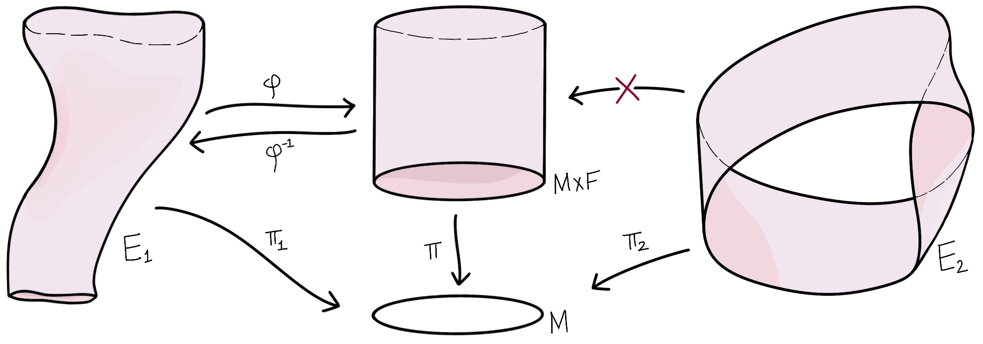
Here, the existence of the homeomorphism $\varphi: E_1 \rightarrow M \times F$ shows that $E_1$ and $M\times F$ are similar in some sense, and the non-existence of one at $E_2$ shows that it is different from the others. For instance, $E_2$ has only a single, connected edge, whereas the cylindrical shapes have two (top and bottom) edges. Mentally, we can think of a homeomorphism between two spaces as the ability to morph one space (as if it were made of extremely malleable clay) into the other without cutting, gluing, or poking holes into it.

The bundle corresponding to $M\times F$ is called the trivial bundle over $M$ having the fiber $F$, and the homeomorphism $\varphi$ is called a trivialization of the bundle $(E_1, M, \pi_1, F)$. By virtue of the existence of $\varphi$, we will write $E_1 \cong M\times F$ (as fiber bundles).

The purpose of introducing the notion of a trivial bundle is that we will demonstrate the following fact: $TG \cong G \times \mathfrak g$. We can trivialize $TG$ in the following way; given a vector $X_g \in T_g G$, we know that $\mathcal L_{g^{-1}*} X_g$ is in $\mathfrak g$. Thus, define the following isomorphism between fiber bundles:

$$\begin{align} \mathcal L:\ TG &\rightarrow G \times \mathfrak g\\ X_g &\mapsto (g, \mathcal L_{g^{-1}*} X_g) \nonumber \end{align}$$

The continuity of $\mathcal L_{g^{-1}*}$ makes the above a valid isomorphism of bundles. If $X\in \mathfrak X^{\mathcal L}(G)$ is a left-invariant vector field that is understood as a smooth section of $TG$, then $\mathcal L$ flattens the section, i.e., each tangent vector $X(g)$ is mapped to the same vector of $\mathfrak g$. We call $\mathcal L$ the left-trivialization of the tangent bundle.

Yet another trivialization is the following:

$$\begin{align} \mathcal R:\ TG &\rightarrow G \times \mathfrak g\\ X_g &\mapsto (g, \mathcal R_{g^{-1}*} X_g) \nonumber \end{align}$$

where $\mathcal R_g (h) = h \odot g$ is the right multiplication by $g$. We said that left/right multiplications lead to equivalent theories, only differing by a sign change. That is typically true of Lie theory, but in this particular case, we will make nontrivial observations by considering both $\mathcal L$ and $\mathcal R$ simultaneously. Consider what happens when we compose $\mathcal R$ with $\mathcal L^{-1}$:

$$\begin{align} \mathcal R \circ \mathcal L^{-1}:\ G \times \mathfrak g &\rightarrow G \times \mathfrak g\\ (g, \tilde X) &\mapsto (g, \mathcal R_{g^{-1}*} \mathcal L_{g*} \tilde X) \nonumber \end{align}$$

This is a bundle endomorphism of $G\times \mathfrak g$ (a homomorphism from it to itself). By construction, it is placing the non-commutativity of $G$ under scrutiny. For each tuple of the form $(g,\tilde X )$, $\mathcal R \circ \mathcal L^{-1}$ makes $\tilde X$ take a ‘round-trip’ by sending it to $T_gG$ via $\mathcal L_{g*}$ and back to $\mathfrak g$ via $\mathcal R_{g^{-1}*}$. Note that $\mathcal R_{g^{-1}*} \mathcal L_{g*} \tilde X=\textrm{Ad}_g\tilde X$. The departure of $\textrm{Ad}_g\tilde X$ from $\tilde X$ is a measure of the non-commutativity of multiplication by $g$. Not all group elements are equally non-commutative; for instance, $e$ commutes with all the other group elements.