Understanding Sparsity through Sub-Gradients

We talked about why sparsity plays an important role in many of the inverse problems that we encounter in engineering. To actually find the sparse solutions to these problems, we add ‘sparsity-promoting’ terms to our optimization problems; the machine learning community calls this approach regularization.

Regularization

An optimization method that was popularized in the $80$s and $90$s is the LASSO , also called $L^1$ norm regularization, which solves problems of the following form:

$$\begin{array}{ll} \underset{x\in \mathbb R^n}{\textrm{minimize}} & g(x) + \lambda \|x\|_1 \end{array}$$

Usually, $g(x)$ corresponds to an error/loss term. It can also be the negative of something we wish to $\text{maximize}$. The claim is that the additional term $\lVert x\rVert_1$ promotes the sparsity of the solution $x^\star$, i.e., it attempts to set one or more elements of $x^\star$ to $0$. Similarly, in ridge regression (also called Tikhonov regularization or $L^2$ norm regularization), we add a $\lVert x\rVert_2^2$ term to the objective. This is known to shrink the solution towards the origin, but it does not necessarily make the solution sparse.¹

What about $\lVert x\rVert_2$ (as opposed to $\lVert x\rVert_2^2$), what would that do? How do we reason about an arbitrary ‘regularization term’ and interpret what it does? If you have encountered this question before, then you’ve likely seen explanations such as this one . 👈🏽 While that’s a great, conversational explainer on sparsity, I want to give it a slightly more formal treatment for anyone interested.

Sub-Gradient Descent

I expect that the reader is familiar with gradient descent and convex functions. I will offer a brief introduction to sub-gradient descent, which extends gradient descent to the case where the objective function is non-differentiable, but still convex.

A non-differentiable function is one that does not have a well-defined gradient at one or more points of its domain. But if the function is convex (i.e., bowl-shaped), then it has the next best thing: a sub-gradient of $f(x)$ at $x^\star$ is a vector $w$, such that the inequality

$$f(x) - f(x^\star) \geq w^\intercal (x-x^\star)$$

holds for all $x$ in the domain of $f$. The sub-gradient $w$ is not unique in general. However, if $f$ is differentiable at $x^\star$, then $w$ takes the unique value of $\nabla f(x^\star)$. A convex function has at least one sub-gradient at every point of its domain; we can prove that fact using this theorem . Observe that sub-gradients can be thought of as hyperplanes that touch or support the function from below, similar to how the gradient of a differentiable convex function touches it from below.

Since the sub-gradient is non-unique, we define the sub-differential of $f$ at $x^\star$, denoted as $\partial f(x^\star)$, as the set of all sub-gradients of $f$ at $x^\star$. We can now do gradient descent, but instead of the gradient, we pick a sub-gradient direction to descend towards. This procedure of sub-gradient descent is motivated by the following fact: $x^\star$ is the global minimizer of $f(x)$ if and only if $\bold 0 \in \partial f(x^\star)$. For differentiable functions, sub-gradient descent reduces to gradient descent.

Similar to how, for differentiable functions,

$$\nabla(f + g)(x)=\nabla f(x) + \nabla g(x),$$

we have

$$\partial (f+g)(x) = \partial f (x) + \partial g(x)$$

However, we are dealing with sets and not vectors in the non-differentiable case. The ‘$+$’ in the preceding equation refers to the Minkowski sum; for sets $\mathcal A$ and $\mathcal B$,

$$\mathcal A + \mathcal B = \left\lbrace a+b | a\in \mathcal A, b \in \mathcal B \right\rbrace$$

Revisiting the LASSO

With this, let’s look at the LASSO-type problem,

$$\begin{array}{ll} \underset{x\in \mathbb R^n}{\textrm{minimize}} & f(x) + g(x) \end{array}$$

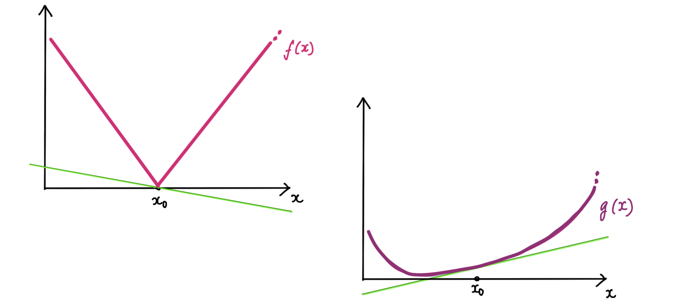
where the green lines show the sub-gradients of the two functions at $x^\star$. This function is minimized whenever we can pick sub-gradients from $f$ and $g$ such that they ‘cancel each other out’.

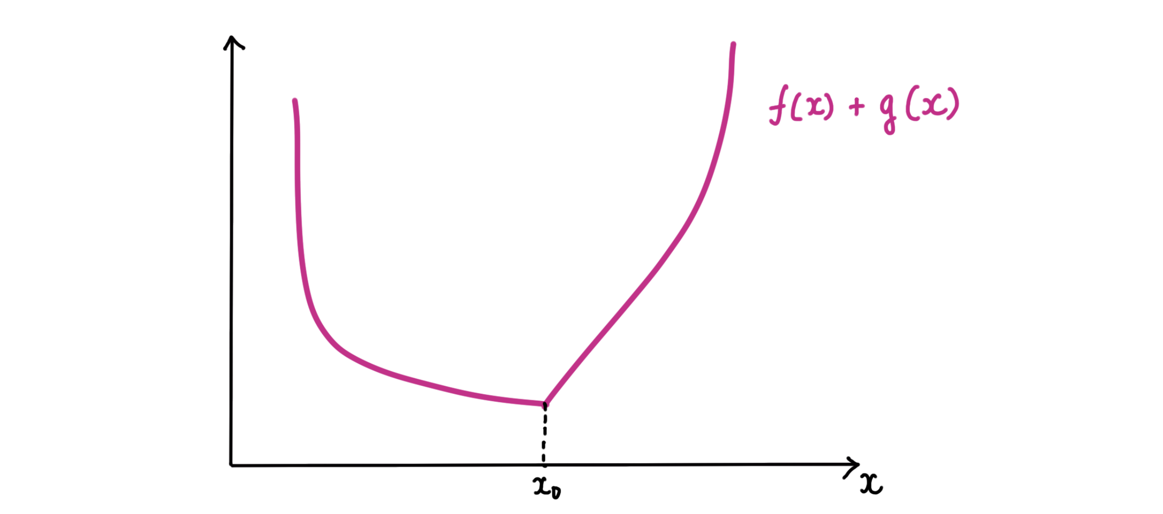
$$f+g\text{ is minimized at }x^\star\\ \Updownarrow \\ \bold 0 \in \partial (f+g)(x^\star) \\ \Updownarrow\\ \exists w \in \partial f (x^\star) \text{ \ such that \ } w+ \nabla g(x^\star) =\bold 0$$

At the differentiable points ($x\neq x^\star$), neither function has much freedom in picking a sub-gradient. But at $x^\star$, $f(x)$ has a range of sub-gradients to pick from; it can choose one that ‘cancels out’ the corresponding (sub-)gradient of $g(x)$ at $x^\star$. This is why a convex, non-differentiable regularization term is likely to pull the solution towards its non-differentiable points!

Choosing a ‘Regularization Term’

Suppose $x\in \mathbb R^2$. The function $\lVert x \rVert_1$ has the following shape:

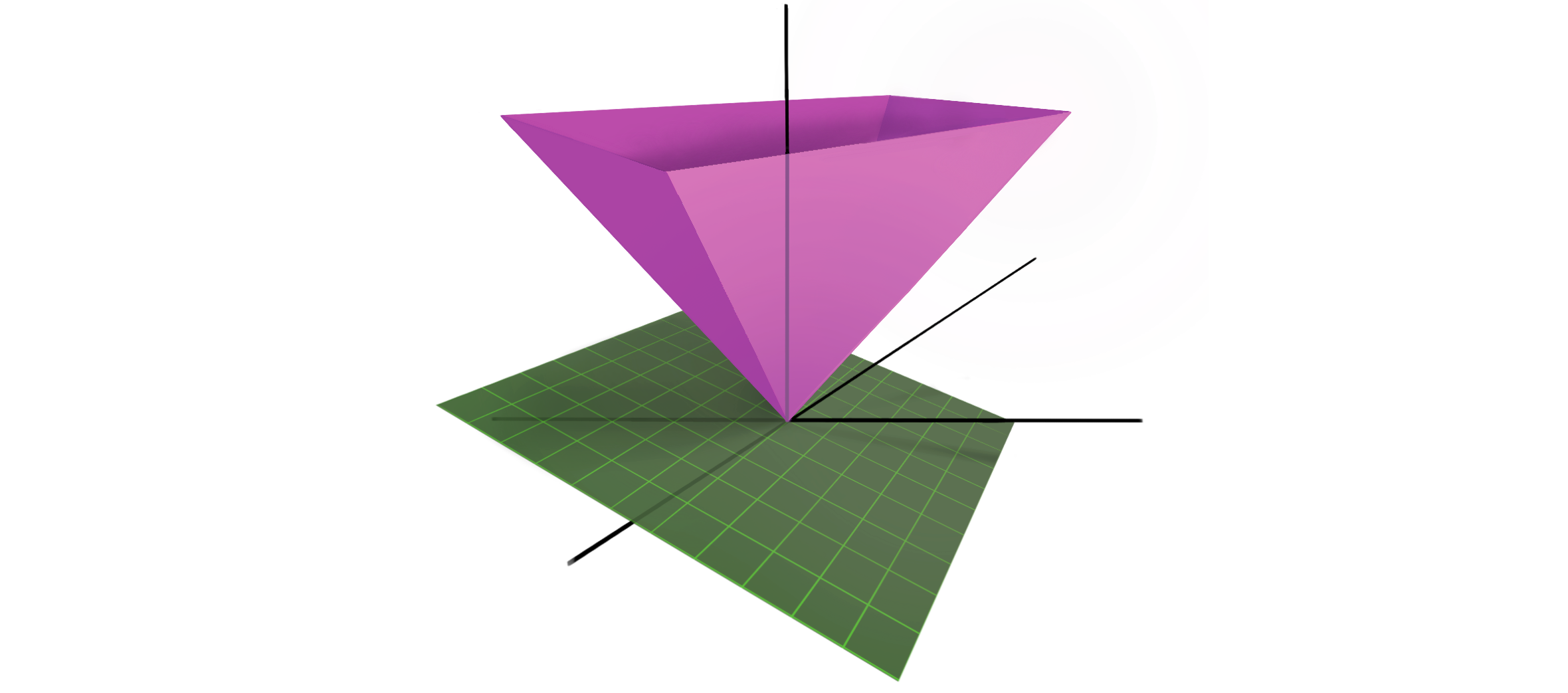
where the green plane is a sub-gradient at the origin. Since $\lVert x \rVert_1$ is non-differentiable along the axes, it tries to snap the minima towards the axes. Note that the axes of $\mathbb R^2$ are exactly where the sparse vectors are. What about when $x\in \mathbb R^3$? At what points is $\lVert x\rVert_1$ non-differentiable then? (Hint: it’s not just the axes!)

The function $\lVert x \rVert_2$ looks like an ice-cream cone:

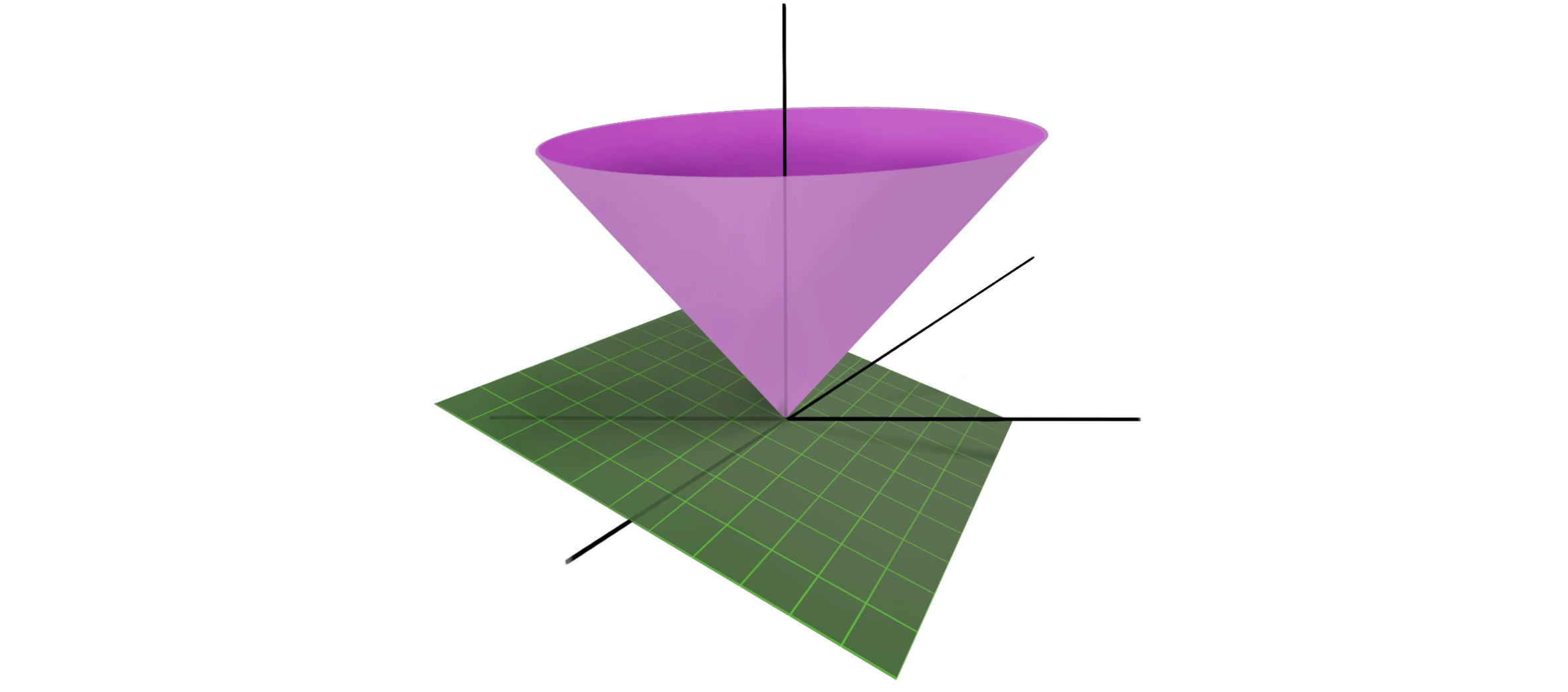
since it’s only non-differentiable at the origin, it tries to snap the solution towards the origin. This is different from ridge regression, which instead uses $\lVert x\rVert_2 ^2$. The function $\lVert x\rVert_2 ^2$ is differentiable everywhere; it is ‘bowl-shaped’. It pulls the solution towards the origin, but does not particularly demand that the solution be exactly $\bold 0$. So is there a use for $\lVert x \rVert_2$? Yes! It can be used to promote the block-sparsity of a vector, where the $0$’s of the vector appear in blocks. Consider

$$x^\intercal = \left[\ x_1^\intercal\ x_2^\intercal\ x_3^\intercal \dots x_n^\intercal\ \right]$$

where $x_i \in \mathbb R^{d_i}$, and $x \in \mathbb R^{\sum_{i=1}^n d_i}$. Suppose we know that the sparsity of $x$ occurs in blocks, i.e., some of the $x_i$ are full of zeros. Then, the regularization term $\sum_{i=1}^{n}\lVert x_i \rVert_2$ is what we want to use since it sets some of the $x_i$ to $\bold 0$ but does not promote sparsity within each block. (I used this fact to solve an engineering problem in my PhD dissertation .)

Closing Note

There are many different ways to think about sparsity. For instance, one could imagine trying to balance a tennis ball that is resting on one of the surfaces we showed above, by holding the surface from below and tilting it. The ball is likely to settle at one of the non-differentiable points of the surface, thereby minimizing its potential energy. I like the sub-gradient interpretation because it works irrespective of the dimension. We can test for differentiability of arbitrary functions even if we cannot visualize them.