Here, I solve Problem $5-5$ from John Lee’s book on Riemannian Manifolds, which demonstrates the non-flatness of the ($2$-)sphere. This problem is particularly interesting because it serves as the motivating example for a later chapter in the book on curvature. As a by-product, we will put to rest the concerns of flat-Earthers.

Connections

First, I go over the technical tools needed to state (let alone solve) the problem. A connection $\nabla$ on a smooth manifold $M$ is a way of differentiating vector fields (and more generally, tensors) along curves in $M$:

\[ \nabla : \mathfrak X(M) \times \mathfrak X(M) \to \mathfrak X(M) \]

where $\mathfrak X(M)$ denotes the space of smooth vector fields on $M$. The axioms/properties that must be satisfied by a connection (specifically, a Koszul connection) can be found in Lee’s book, so I will focus on the insights.

We write $\nabla X: \mathfrak X(M) \rightarrow \mathfrak X(M)$ to denote the total covariant derivative of $X$, with the intention that $\nabla X(Y) = \nabla _Y X$ inserts $Y$ into the first slot of $\nabla$. Compare this with the map $\nabla _X:\mathfrak X(M) \rightarrow \mathfrak X(M)$ which inserts $Y$ into the second slot of $\nabla$. The former is $C^\infty(M)$-linear in $Y$, while the latter is $\mathbb R$-linear but not $C^\infty(M)$-linear in $Y$. That is, we have $C^\infty(M)$-linearity in the first slot:

\[ \nabla X (fY) = \nabla _{fY} X = f \nabla X (Y) \]

but a product/Leibnitz rule in the second slot:

\[ \nabla _X (fY) = X(f) + f \nabla _X Y \]

Since the total covariant derivative $\nabla X$ is $C^\infty(M)$-linear, it is a tensor, but the connection itself is not a tensor.

The Levi-Civita Connection

There is a lot of freedom in choosing a connection on a Riemannian manifold. Once chosen, a connection specifies a rule for ‘connecting’ the nearby tangent spaces (or more generally, fibers of a vector bundle) of the manifold, thereby defining a notion of differentiation of vector fields. The fundamental theorem of Riemannian geometry says that there exists a unique connection, called the Levi-Civita connection, that satisfies the following properties:

1. Metric Compatibility: $\nabla _X \langle Y, Z \rangle = \langle \nabla _X Y, Z \rangle + \langle Y, \nabla_X Z \rangle $
2. The Torsion-Free Property/Symmetry: $ \nabla _X Y - \nabla _Y X = [X, Y]$

The first of these can be viewed as a Leibniz/product rule for the metric¹. The second property is a bit more mysterious; I like to think that Property 2 is about the compatibility of the connection with the flows (and thus, the differential structure) of $M$, whereas Property 1 is about compatibility with the geometry. The following discussion will shed more light into torsion-free connections.

Comparison with the Lie Derivative ($\mathcal L_X$)

As suggested in the aside (the indented grey box) above, the connection defines a derivative of $C^\infty (M)$ functions in the following sense:

\[ \nabla _X f = \mathcal L_X f = X(f) \in C^\infty (M) \]

which is also the same as $df(X)$, $d$ being the exterior derivative. So, $\nabla _X$ and $\mathcal L_X$ operate similarly on functions. However, $\nabla _X Y \neq \mathcal L_X Y$ (in general) when $Y \in \mathfrak X(M)$. This was for me one of the biggest conceptual difficulties while self-studying Riemannian geometry, so it is worth dwelling on the point.

Recall that

\[ \mathcal L_X Y(f) = [X, Y](f) = X\big(Y(f)\big) - Y\big(X(f)\big) \]

which means that $\mathcal L_X Y = [X, Y]$ is simply the Lie bracket of vector fields. We observe the following points of departure between $\nabla _X Y$ and $\mathcal L_X Y$:

• The Lie derivative is well-defined once a smooth structure for $M$ is specified, whereas the connection is an additional structure that is imposed on $M$; in particular, endowing $M$ with geometry uniquely specifies the Levi-Civita connection. Importantly, there is no natural choice of a connection on a smooth manifold until a metric is chosen for it

• The Lie derivative $\mathcal L_X Y$ at $p\in M$ is defined via local flows/diffeomorphisms of $X$ near $p$, whereas $\nabla _X Y$ only depends on the vector $X_p \in T_p M$

• $X \mapsto \mathcal L_X$ is only an $\mathbb R$-linear map (and therefore, not a tensor), whereas $X \mapsto \nabla_X$ is $C^\infty(M)$-linear². Neither of $\mathcal L_X(\hspace{1pt}\cdot\hspace{1pt})$ and $\nabla_X(\hspace{1pt}\cdot\hspace{1pt})$ is $C^\infty(M)$-linear

• If $\nabla$ is torsion-free, then the torsion-free condition can be rearranged to yield

\[ \nabla_ X Y = \big(\nabla X + \mathcal L_ X\big) Y \]

The first of these is a $C^\infty(M)$-linear transformation of $Y$, so $\nabla _X$ can be viewed as an affine transformation, with $\mathcal L_X$ playing the role of translation. The presence of $\mathcal L_X$ destroys the linearity of $\nabla _X$, until and unless $X$ and $Y$ commute, in which case $\mathcal L_X Y = [X, Y] \equiv 0$.

Tangential Connection

In general, the connection is given with respect to a smooth local frame $({E_i})_{i=1}^n$ on $U\subseteq M$ by $\nabla _{E_i} E_j = \Gamma_{ij}^k E_k$, where $\Gamma_{ij}^k$ are called the Christoffel symbols of the connection with respect to $(E_i)_{i=1}^n$, and Einstein summation is implied. The Christoffel symbols specify the action of $\nabla$ on arbitrary vector fields on $U$:

\[ \nabla_X Y = X(Y^i) E_i + Y^i \nabla_X E_i = \big(X(Y^k) + X^i Y^j \Gamma_{ij}^k \big)E_k \]

where $Y = Y^i E_i$ is the expansion of $Y$ in the frame $(E_i)_{i=1}^n$. The Christoffel symbols $\Gamma_{ij}^k$ of the Levi-Civita connection can be expressed using the second Christoffel identity (which relies on coordinates) or by using the Koszul formula (which is coordinate-free); see Corollary $5.11$ in Lee’s book (on Riemannian manifolds).

Sometimes, a more straightforward way to work with the Levi-Civita connection is to isometrically embed $M$ in a higher-dimensional Euclidean space, and then (in a sense) pull back the Euclidean connection to $M$. This is considered the extrinsic approach and comes at the risk of obscuring the intrinsic structure of $M$. Let $\mathbb R^{\bar n}$ be the Euclidean $\bar n$-space having the Euclidean metric $\bar g$. Its Levi-Civita connection is given by

\[ \overline \nabla_X Y = X(Y^i) \frac{\partial}{\partial x^i} \]

which is precisely how a naive calculus student would differentiate vector fields – the Riemannian geometer should be aware that this formula only holds because the Christoffel symbols are all $0$ in this case.

Now, let $\pi: T_p \mathbb R^{\bar n} \rightarrow T_p M$ be the orthogonal projection of tangent vectors of $\mathbb R^{\bar n}$ onto $T_p M$. Then, the Levi-Civita connection on $M$, denoted $\nabla$, is given by

\[ \nabla_X Y = \pi \left(\overline \nabla_{\overline X} \overline Y\right) \]

where $\overline X$ and $\overline Y$ are smooth extensions of $X$ and $Y$ to an open set of $\mathbb R^{\bar n}$, respectively. This paints an extrinsic picture of the covariant derivative: it is the rate of change of $Y$ along $X$ as seen from within $M$, i.e., changes in $Y$ that are normal to $M$ are disregarded.

---

We are ready to attempt Problem $5-5$ from Lee’s book.

The Sphere

A vector field $X$ is said to be a parallel vector field if $\nabla X$ is identically $0$. A (local) parallel coordinate frame (see my other post for an introduction to coordinate frames) exists on (an open set of) a manifold $M$ if and only if $M$ is (locally) flat. Here, local (or global) flatness refers to the property of being locally (or globally) isometric to an open set of the Euclidean space of the same dimension.

A $2$-dimensional manifold is locally flat if and only if a small piece (i.e., an open set) cut out from it can be laid flat on the table without stretching, tearing, or crumpling it. The surface of a Cylinder and the Möbius strip (with a certain, natural choice of metric for it) are examples of locally flat surfaces; this is exactly why one can construct these surfaces from a piece of paper. The crux of Problem $5-5$ is to show that such a local parallel vector field does not exist on the sphere $S^2$. (This can be compared to the difficulty of drawing a map of the Earth that does not introduce distortions of some sort.)

First, Lee asks us to consider the following embedding of the $2$-sphere in $\mathbb R^3$:

\[ \begin{aligned} \psi: U &\rightarrow \mathbb R^3 \\ (x^1, x^2) &\mapsto \left(\sin x^1 \cos x^2, \sin x^1 \sin x^2, \cos x^1\right) \end{aligned} \]

where $U\subseteq S^2$ is an open set on the sphere and $(x^1, x^2)$ are the usual spherical polar coordinates on the sphere; technically, $\psi$ is the pullback of an embedding under the spherical polar parameterization:

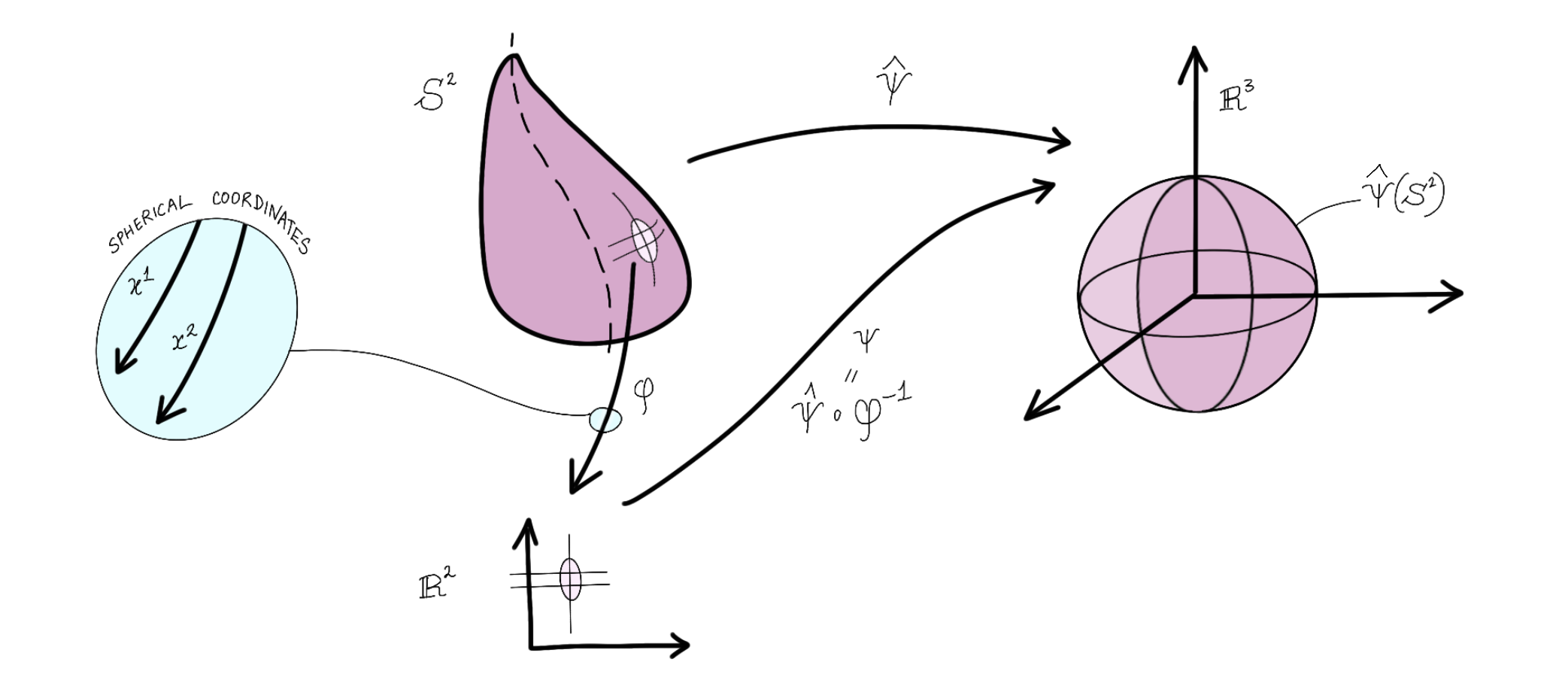
In the illustration, we use a ‘wobbly sphere’ to remind us that $S^2$ does not necessarily come endowed with geometry. Rather, by treating $\hat \psi$ as an isometry, we will ‘pull back’ the geometry of $\mathbb R^3$ onto $S^2$. To this end, consider the frame $\big(\frac{\partial}{\partial x^1}, \frac{\partial}{\partial x^2}\big)$ on $\mathbb R^2$³. We know that $\varphi ^{-1}$ pushes this forward, yielding the local coordinate frame $(\varphi ^{-1}_*\frac{\partial}{\partial x^1},\varphi ^{-1}_*\frac{\partial}{\partial x^2})$ on $S^2$. It can then be pushed forward to $\mathbb R^3$, giving us

\[ \Big(\hat \psi_*\big(\varphi ^{-1}_*\frac{\partial}{\partial x^1}\big), \hat \psi_*\big(\varphi ^{-1}_*\frac{\partial}{\partial x^2} \big) \Big) = \Big(\psi_*\frac{\partial}{\partial x^1}, \psi_*\frac{\partial}{\partial x^2} \Big). \]

Denote the standard frame in $\mathbb R^3$ by $(\frac{\partial}{\partial y^1}, \frac{\partial}{\partial y^2}. \frac{\partial}{\partial y^3})$. We have (using the usual chain rule),

\[ \begin{aligned} X \coloneqq \psi_* \frac{\partial}{\partial x^1} &= \cos x^1 \cos x^2 \frac{\partial}{\partial y^1} + \cos x^1 \sin x^2 \frac{\partial}{\partial y^2} - \sin x^1 \frac{\partial}{\partial y^3}, \\ Y \coloneqq \psi_* \frac{\partial}{\partial x^2} &= -\sin x^1 \sin x^2 \frac{\partial}{\partial y^1} + \sin x^1 \cos x^2 \frac{\partial}{\partial y^2}. \end{aligned} \]

So, there is a good reason for distinguishing between $(x^1, x^2)$ and $(y^1, y^2, y^3)$. The second of these vector fields is $Y = -y^2 \frac{\partial}{\partial y^1} + y^1 \frac{\partial}{\partial y^2}$, and the first is more complicated to write in terms of $(y^1, y^2, y^3)$.

Are $X$ and $Y$ Parallel?

If they are, then we will conclude that the sphere is flat.

Observe that $X$ are the longitudinal (i.e., vertical) vector fields on the sphere, and $Y$ are the latitudinal (i.e., horizontal) vector fields. Lee asks us to compute $\nabla_{X} X$ and $\nabla_{Y} X$ to assess the parallel-ness of $X$, with $\nabla$ being the tangential connection. I tried this using the standard (Cartesian) coordinate frame of $\mathbb R^3$, but the computations are cumbersome. For instance, we have

\[ \begin{align*} \overline \nabla_{\overline Y} {\overline X} &= {\overline Y}({\overline X}^1) \frac{\partial}{\partial y^1} + {\overline Y}({\overline X}^2) \frac{\partial}{\partial y^2} + {\overline Y}({\overline X}^3) \frac{\partial}{\partial y^3}\\ &= \overline Y\left(\frac{y^3 y^1}{\sqrt{{y^1}^2 + {y^2}^2}}\right)\frac{\partial}{\partial y^1} + \overline Y\left(\frac{y^3 y^2}{\sqrt{{y^1}^2 + {y^2}^2}}\right)\frac{\partial}{\partial y^2} \\ &\qquad + \overline Y\left(-\sqrt{{y^1}^2 + {y^2}^2}\right)\frac{\partial}{\partial y^3}\\ &= \frac{-y^2 y^3}{\sqrt{{y^1}^2 + {y^2}^2}}\frac{\partial}{\partial y^1} + \frac{y^1 y^3}{\sqrt{{y^1}^2 + {y^2}^2}}\frac{\partial}{\partial y^2} \end{align*} \]

Even without projecting onto the sphere (recall the definition of a tangential connection), we see that $\overline \nabla_{\overline Y} {\overline X}$ is $0$ when $y^3=0$, meaning that $X$ is parallel along the equator of the sphere. The computation of $\overline \nabla_{\overline X} {\overline X}$ can also be done in this way, but it will be messy. Let’s look for a better approach.

Before we get there, what do you think $\nabla _X X$ will turn out to be? Here’s a hint: the integral curves of $X$ are said to be geodesics (locally length-minimizing paths) if and only if $X$ is parallel along its integral curves, i.e., $\nabla _X X = 0$. What are the geodesics of the sphere? You might know these as the paths that airplanes like to take when flying long distances.

Using a Coordinate Frame

The frame $\left(\frac{\partial}{\partial y_1}, \frac{\partial}{\partial y_2}, \frac{\partial}{\partial y_3}\right)$ is a global coordinate frame for $\mathbb R^3$ derived from the standard/trivial coordinates, $(y^1,y^2, y^3) \mapsto (y^1,y^2, y^3)$. It is attractive to us because it is orthonormal (the metric tensor coefficients are $\delta_{ij}$, making the metric reduce to a dot product), and the Christoffel symbols $\lbrace\Gamma_{ij}^k\rbrace_{i,j,k=1}^3$ of the Levi-Civita connection $\overline \nabla$ are all identically $0$.

Let’s construct a different coordinate frame for $\mathbb R^3$. We consider the spherical polar parametrization of $\mathbb R^3$, $(\varphi, \theta, r) \mapsto (r \sin \varphi \cos \theta, r \sin \varphi \sin \theta, r \cos \varphi)$. This induces a coordinate frame $(\partial_\varphi, \partial_\theta, \partial_r)$ with $\partial_\varphi\vert_{r=1}=X$ and $\partial_\theta\vert_{r=1}=Y$; the vertical line ‘$\vert$’ is read as ‘restricted to’. This frame is not defined along the $y^3$ axis, but that’s okay – it is a local coordinate frame.

It seems as if this should simplify the calculation greatly, so (by an application of the no free lunch theorem ) there must be a catch. The catch is that the frame $(\partial_\varphi, \partial_\theta, \partial_r)$ is not orthonormal, so we need to compute the Christoffel symbols of the Levi-Civita connection with respect to this frame. (Chapter 7 of Lee shows that a local orthonormal coordinate frame can exist if and only if the manifold is locally flat; this is yet another way of demonstrating the non-flatness of the sphere.)

Let’s look at the metric tensor coefficients $g_{ij}$. We have, $g_{11}=\langle \partial_\varphi, \partial_\varphi \rangle$, with

\[ \begin{align} \partial_\varphi &= r \cos \varphi \cos \theta \frac{\partial}{\partial y^1} + r \cos \varphi \sin \theta \frac{\partial}{\partial y^2} - r \sin \varphi \frac{\partial}{\partial y^3}\\ \partial_\theta &= -r \sin \varphi \sin \theta \frac{\partial}{\partial y^1} + r \sin \varphi \cos \theta \frac{\partial}{\partial y^2}\\ \partial_r &= \sin \varphi \cos \theta \frac{\partial}{\partial y^1} + \sin \varphi \sin \theta \frac{\partial}{\partial y^2} + \cos \varphi \frac{\partial}{\partial y^3} \end{align} \]

so that $g_{11}(\varphi, \theta, r) = r^2$. Completing the metric tensor, we find that $g_{22}(\varphi, \theta, r) = r^2 \sin^2 \varphi$ and $g_{33}(\varphi, \theta, r) = 1$. Amazingly (but as expected), $g_{12}$, $g_{13}$, $g_{23}$, and their symmetric counterparts are all identically $0$.⁴ The Christoffel symbols in a coordinate frame are given by the formula

\[ \begin{align} \Gamma_{ij}^k &= \frac{1}{2} g^{kl} \left( \partial_i g_{jl} + \partial_j g_{il} - \partial_l g_{ij} \right) \end{align} \]

where $g^{ij}$ are coefficients of the inverse of the metric tensor (see p. 123 of Lee). So, we have

\[ \begin{align} \Gamma_{11}^3 = -r, \quad \Gamma_{12}^2=\frac{\cos \varphi}{\sin \varphi}, \quad \Gamma_{13}^1 = \frac{1}{r}. \end{align} \]

giving us

\[ \begin{align} \overline \nabla_{\overline X} \overline X &= \overline \nabla_{\partial_\varphi} \partial_\varphi \\ &= \overline \nabla_{\partial_1} \partial_1 =\Gamma_{11}^3 \partial_3 = -r \partial_r \end{align} \]

Since $\overline \nabla_{\overline X} \overline X$ is purely in the radial direction, we have that $\nabla _X X = \pi \left(\overline \nabla_{\overline X} \overline X\right) =0$. Thus, $X$ is indeed parallel along its own integral curves; the integral curves of $X$ are segments of the geodesics (i.e., great circles) passing through the poles.

Lastly, we compute $\nabla _Y X$ in the new frame:

\[ \begin{align} \overline \nabla_{\overline Y} \overline X &= \overline \nabla_{\partial_\theta} \partial_\varphi \\ &= \overline \nabla_{\partial_2} \partial_1 = \Gamma_{21}^2 \partial_2 = \frac{\cos \varphi}{\sin \varphi} \partial_\theta\\ \Rightarrow \nabla_{Y} X &= \pi \left( \overline \nabla_{\overline Y} \overline X\right )=\frac{\cos \varphi}{\sin \varphi} \partial_\theta \end{align} \]

(since $\Gamma_{21}^2=\Gamma_{12}^2$ for the Levi-Civita connection). As we deduced before, $X$ is only parallel in the horizontal/latitudinal directions if $\cos \varphi =0$, i.e., at the equator. In conclusion, $\nabla X \neq 0$.

Could there be another parallel frame?

We have only shown that $(X,Y)$ is not a parallel frame, which does not preclude the existence of another parallel coordinate frame. Lee asks us to consider the point $(y^1, y^2, y^3)=(1,0,0)$ in $\mathbb R^3$, and show that there is no parallel coordinate frame near this point. By symmetry, the argument would extend to other points on the sphere. I omit the arguments here, but page $194$ of Lee’s book outlines the process of constructing a parallel frame near $p=(1,0,0)$. The key idea is that such an attempt to construct a parallel vector field would both (i) coincide with $X$, and (ii) fail to be parallel.

---

Some Stronger Claims

In the above, we worked with a specific isometric embedding of the sphere in $\mathbb R^3$, restricting our investigation to a specific choice of a metric. Could another metric be prescribed for the sphere that makes it flat (or equivalently, enables us to prescribe a local orthonormal/parallel coordinate frame)? Firstly, we belabor the point that flatness is dependent on the metric at all.

The non-flat torus: The 2-torus $\mathbb T^2 \cong S^1 \times S^1$ can be embedded in $\mathbb R^3$ as a donut: this is not flat, because parallel transport of a vector from inside the hole (i.e., close to the axis) of the donut to the outside (i.e., far from the axis) would need to preserve its length, posing an obstacle to the construction of a parallel coordinate frame. Equivalently, one cannot wrap a piece of paper around a donut (unless the length or width of the piece of paper were vanishingly small) without introducing creases or folds in the paper.

The flat torus: At the same time, the 2-torus can be embedded in $\mathbb R^4$ (analogous to how a circle can be embedded in $R^2$⁵) or realized as the quotient manifold $\mathbb R^2/\mathbb Z^2$. The latter two constructions would give rise to natural choices of flat metrics. We conclude that $\mathbb T^2$ admits a flat metric, but the donut (which is $\mathbb T^2$ with a specific choice of metric) is not flat. That being said, it is possible to isometrically embed the flat torus in $\mathbb R^3$; these researchers are working on visualizing such an embedding, and observe that it has a self-similar, fractal-like structure, indicating that the situation is much more subtle than our naive conception of the donut.

The locally flat sphere: The sphere does admits a metric that is locally flat (near a given point, $p\in \mathbb S^2$). To see this, we take a cube in $\mathbb R^3$ and smooth all of its edges and corners (to make it smooth); this smoothed cube is now a smooth embedding of the sphere in $\mathbb R^3$, and its pullback metric is certainly (locally) flat near some of the points. So, a more appropriate question to ask is whether the sphere can be globally flat, i.e., does it admit a metric that is flat in every neighborhood, even near the ’edges’ of the smoothed cube?

The (non-existence of a) globally flat sphere: Surprisingly, the answers to such questions come from algebraic geometry, having their roots in combinatorics (i.e., counting arguments). The Euler characteristic of the sphere, combined with the Gauss-Bonnet theorem can be used to show that the sphere does not admit a globally flat metric. Here’s another proof that relies on a theorem that may be familiar (or at least accessible) to most readers. Let $(S^2, g)$ be a hypothesized flat metric on the sphere. There exists then, a global parallel vector field $X$. By metric compatibility of the corresponding Levi-Civita connection, we have

\[ \nabla_Y \langle X,X \rangle = \langle \nabla_Y X, X \rangle + \langle X, \nabla_Y X \rangle = 0 \]

This means that if $\langle X, X\rangle _p \neq 0$ at some point $p$, then $\langle X, X\rangle$ (and therefore, $X$) does not vanish anywhere on $S^2$. The hairy ball theorem says that this is impossible – a contradiction.

---

A Word of Caution!

The most confusing part of self-learning Riemannian geometry has been, for me, the conflation between frames and coordinate frames. I suggest that the reader familiarizes theirself with the definition of either (a coordinate chart induces a frame, but not every frame is the frame derived from a coordinate chart). Every time you encounter a formula, statement, or theorem, take care to check whether it only holds for a coordinate frame.

The following examples show why this distinction is important:

• The left-invariant vector fields $(E_i)_{i=1}^n$ of a Lie group form a global, orthonormal (after carrying out the Gram-Schmidt process) frame. Does this mean that every Lie group is globally flat? No, because the frame of left-invariant vector fields on a non-Abelian Lie group is not a coordinate frame. To see this, observe that $[E_i, E_j] \neq 0$ whereas the Lie brackets must vanish in a coordinate frame (since the partial derivative operators of $\mathbb R^n$ commute).⁶

• For the same reason, it is seldom possible to choose an orthonormal coordinate frame. One either gives up orthonormality (choosing to introduce a metric tensor) or gives up the coordinate frame (choosing to work with a frame that is not a coordinate frame, such as $(E_i)_{i=1}^n$).

• The Christoffel symbols of the Levi-Civita connection are symmetric in the lower indices ($\Gamma_{ij}^k = \Gamma_{ji}^k$), but this is only true in a coordinate frame.

• The identity we used to compute the Christoffel symbols in this post only holds in a coordinate frame. In a non-coordinate frame, we would replace it with the appropriate formula in Corollary 5.11 of Lee’s book.