Let’s look at the norm balls corresponding to the different $p$-norms in $\mathbb R^n$, where $n$ is the dimension of the space. For a vector $v\in \mathbb R^n$, the $p$-norm is
\[ \|x\|_p \coloneqq \left(\sum_i |x_i|^p\right)^{\frac{1}{p}} \]
When $p=2$ this is the usual Euclidean distance. The corresponding ball is what we think of when someone says ball, it is all the points that are within a given distance from the origin. More generally, the ball of ‘radius’ $r$ corresponding to a norm $\lVert{}\cdot{}\rVert$ is
\[\lbrace x\ |\ x\in\mathbb R^n, \|x\|\leq r\rbrace\]
Let’s call the ball corresponding to $\lVert{}\cdot{}\rVert_p$ as the $p$-ball. If $r=1$, we will call it a unit ball. This website shows the unit balls corresponding to other $p$-norms. Here is my artistic illustration of the same:
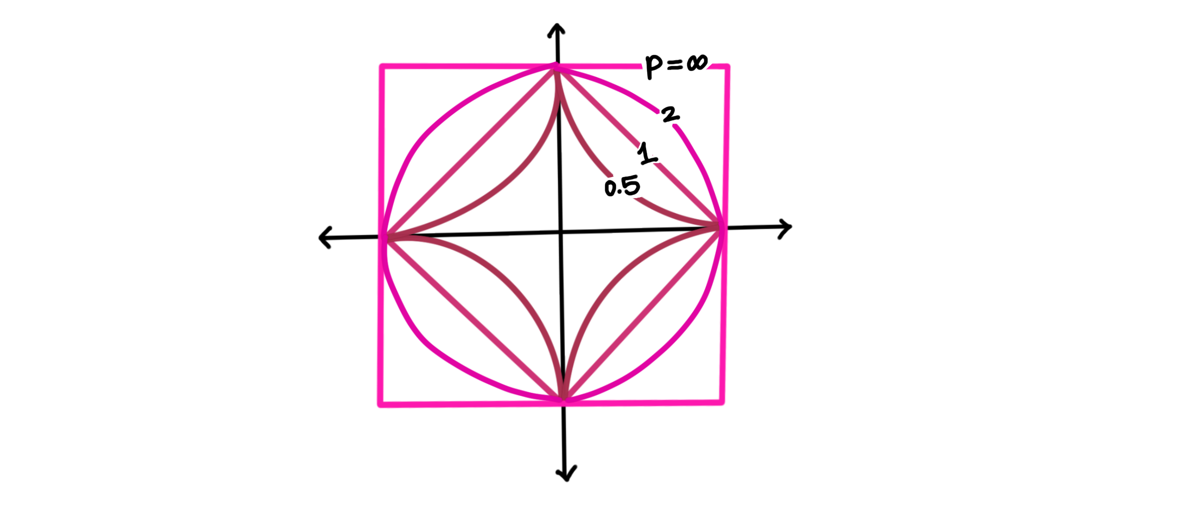
The figure may indicate that $\lVert{}\cdot{}\rVert_p$ gets bigger as $p$ increases, but it’s the other way around:
\[\|x\|_1 \geq \|x\|_2 \geq \dots \geq \|x\|_\infty\]
because you need to go further from the origin to get to the $\infty$ ball. This is similar to how a car with a poorer mileage would need to expend more fuel to get to the same point. So the balls get bigger, but the ‘mileage’ gets smaller.
If $p<1$, then the corresponding “$p$-norm” is not actually a norm, as it is guaranteed to violate the conditions which we usually place on a norm. What feature do we see appearing in the $p$-balls, when $p<1$? The answer is that they curve inwards (are non-convex). In particular, the $0$-ball is quite bizarre, it is exactly the axes! ( Recall that the “$0$-norm” counts the number of non-zero elements in a vector, which is $1$ for each point on the axes). Let’s not talk about the $0$-ball for now.
The $2$-Ball
When $n=2$ the $2$-ball is a circle, and when $n=3$ the $2$-ball is a sphere. What’s less obvious is the case of $n=1$, in which case each of the $p$-norm unit balls is just the line segment from $-1$ to $1$.
We may or may not remember from high-school physics that spheres (i.e., $2$-balls) minimize the ratio of the surface area to volume of a shape. It is why bubbles take spherical shapes, in order to minimize their potential energy. A defining feature of the $2$-ball is that it has continuous rotational symmetry – we can rotate the $2$-ball without changing its shape, something we cannot do for any of the other $p$-balls.
The $\infty$-Ball
Recall that the $\infty$-norm is evaluated by taking the limit $p\rightarrow \infty$ in the definition of the $p$-norm, giving
\[ \|x\|_\infty=\max\left\lbrace|x_1|, |x_2|, \dots, |x_n|\right\rbrace \]
The $\lVert{}\cdot{}\rVert_\infty$ unit ball is always a cube in each dimension, it can be treated as the definition of a unit cube. As such, it has $2n$ faces in dimension $n$. This is because
\[ \max\left\lbrace|x_1|, |x_2|, \dots, |x_n|\right\rbrace \leq 1 \] \[ \Updownarrow \] \[ |x_1|\leq 1\quad \text{and}\quad |x_2|\leq 1\quad \text{and}\quad \dots\quad |x_n|\leq 1 \] \[ \Updownarrow \] \[ x_1\leq 1\quad \text{and}\quad -x_1\leq 1\quad \dots\quad x_n\leq 1 \quad \text{and}\quad -x_n\leq 1 \]
which gives us $2n$ linear constraints, with each linear constraint adding a face.
The $1$-Ball
The $1$-Ball in $2$ dimensions seems like a rotated square, or a diamond, and it appears like this should generalize. Let’s count its faces.
\[ |x_1| + |x_2| + \dots + |x_n| \leq 1 \quad \Leftrightarrow \quad \pm x_1 \pm x_2 \pm \dots \pm x_n \leq 1 \]
where each ‘$\pm$’ indicates that we can choose either sign to obtain a different inequality. The total number of linear inequalities that we can construct is $2^n$. So $1$-balls have many, many more faces than $\infty$-balls in higher dimensions!
This observation has consequences in the field of optimization; some poor bloke here is trying to check whether a given vector $x$ lies inside the $1$-ball. They write this out as a system of linear inequalities, only to realize that it would take an exponentially large number of linear inequalities to do this.
Equivalence of Norms
Given any two numbers $p_1$ and $p_2$ between 0 and $\infty$, with $1\leq p_1,p_2\leq \infty$, we can place $p_1$-balls inside and outside a given $p_2$-ball so that they touch. Two examples of this are as follows:
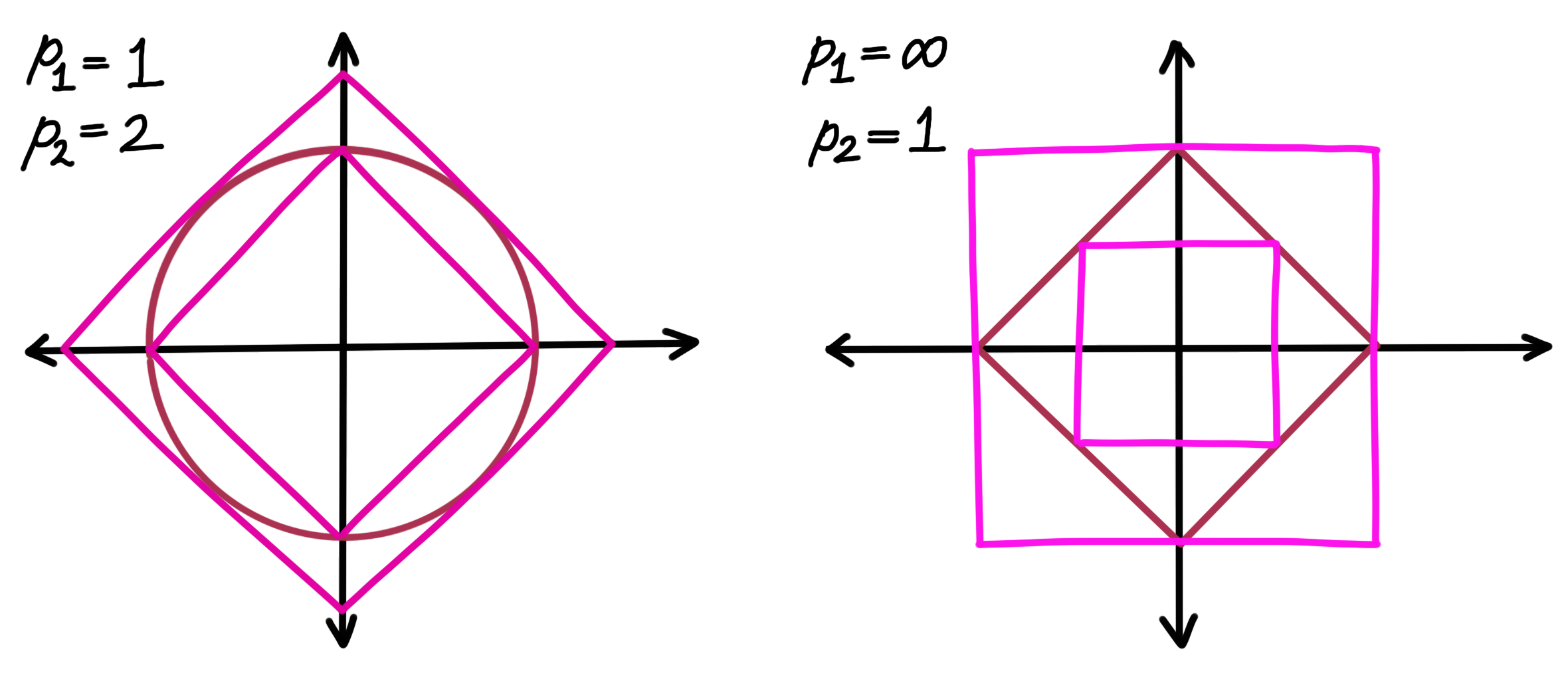
This is what is meant when we say that the $p$-norms are equivalent. Vectors are big (or small) in one norm if and only if they’re big (or small) in the other. ‘Big’ and ‘small’ are used very subjectively here.
Higher Dimensions
We can use everything we just introduced to show interesting quirks of high-dimensional geometry. While this is an entertaining discussion in its own right, it has important consequences in fields like deep learning and probability theory.
The Construction: Consider placing a cube of side length $2$ centred at the origin, as well as a green cube with side length $4$. Then place a sphere at each of the corners of the (inner) cube so that they touch each other, as follows:
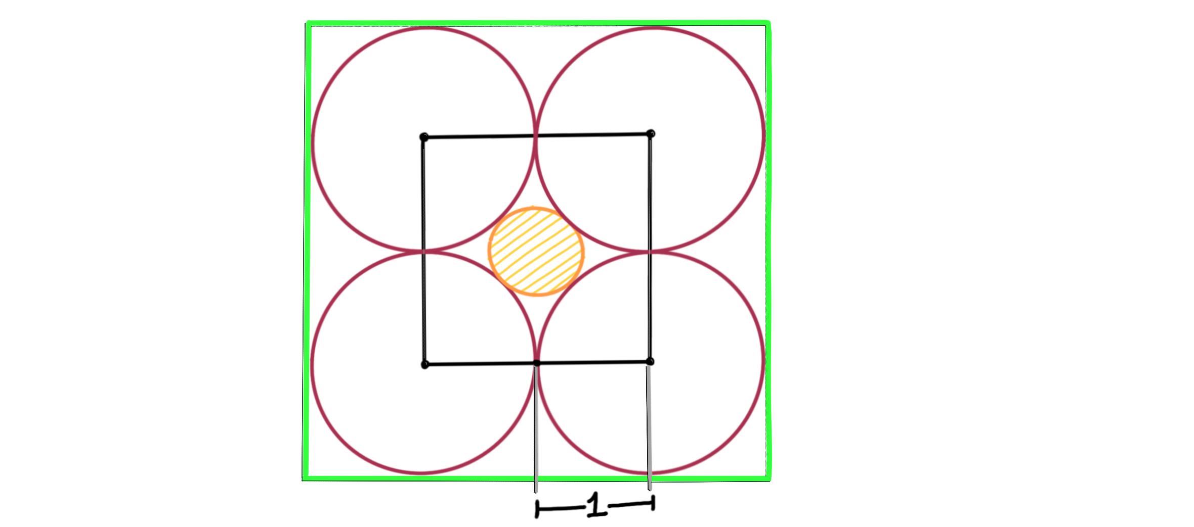
where by ‘sphere’ and ‘cube’ we really mean hypersphere and hypercube, which are their corresponding higher dimensional analogues. Finally, we try to squeeze in a new orange sphere at the centre. The entire configuration fits snugly inside the bigger green cube, and the maroon/pink spheres are in some sense ’tightly packed’ inside the green cube. The figure above is for dimension $2$.
Some Observations: Let’s say we are in some higher dimension, $n$. If this feels like unfamiliar territory, we can think of these as $2$-balls and $\infty$-balls, so we have all the machinery needed to be able to think about these objects at some capacity. For example, we know the following:
- From the origin, we can travel exactly $1$ unit along any axis to reach the inner cube
- The radii of the spheres at the corners is $1$
- The corners of the inner cube are $\sqrt n$ away from the origin, in terms of the Euclidean distance (or by a repeated application of the Pythagoras theorem )
When $n\gg1$, the corners of the inner cube are extremely ($\sqrt n$) far from the origin, whereas its faces are still $1$ unit away. People often phrase this as “higher dimensional cubes are spiky”. Here are some weirder facts:
- The spheres at the corners still have radius $1$
- There are $2^n$ spheres at the corners, because there are $2^n$ corners for the cube
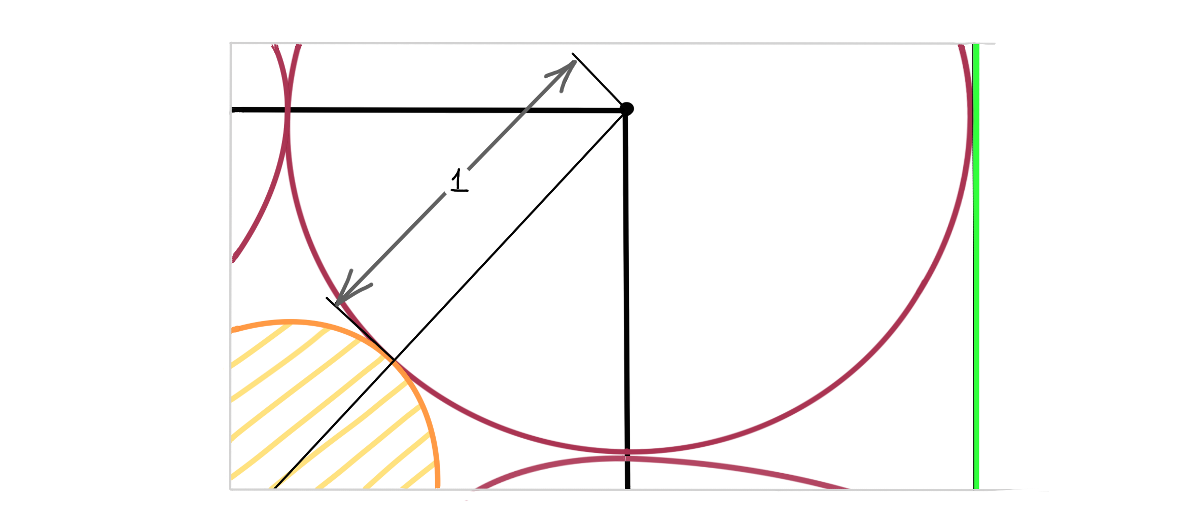
- The orange sphere has a radius of $\sqrt n -1$
Thus, in $1$ dimension, the orange sphere has radius $0$. In $3$ dimensions it has radius $\sqrt 3 -1$. In $4$ dimensions it has radius… $1$? It’s the same size as the spheres at the corners… and it touches the faces of the inner cube…
- In the $10^{th}$ dimension, the sphere in the middle sticks out of the outer (green) cube!
Because the corners of the cube have moved far from the origin, so have the unit spheres we placed at them, making more room for the orange sphere to expand with the dimension.
Going Inwards
Let’s take now the following construction, where we inscribe a purple sphere inside the inner cube. These are precisely the unit balls of the $2$ and $\infty$ norms:
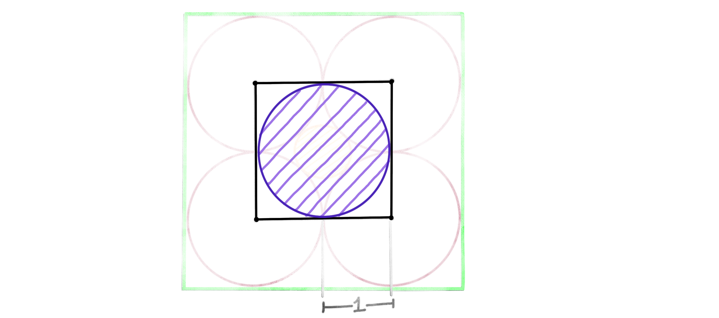
We saw that the $\infty$-ball always touches the $2$-ball from the outside, so even if we turn up the dimension, the sphere better remain contained within the cube. But the corners are still moving away from the origin, so the cube seems to be getting comparatively larger. Let $\text{Vol}({}\cdot{})$ denote the volume (given by the Lebesgue measure ) of a set.
\[\frac{\text{Vol}\left(\textit{\ Unit Sphere in }\mathbb R^n\ \right)}{\text{Vol}\left(\textit{\ Unit Cube in }\mathbb R^n\ \right)}\ \rightarrow\ 0\qquad \text{as}\ n\rightarrow \infty \]
The higher dimensional sphere is insignificantly small in comparison to the cube. Actually, our earlier construction was also saying the same thing. The purple sphere can be thought of as one of the spheres we placed at the corners of the inner cube, each of which vanishes as $n\rightarrow \infty$!1
There’s a variety of ways of showing this, though it’s less straightforward than the stuff we did so far. My favorite proof of this (or rather, a comparable) result is from example $2.2.5$ of Rick Durett’s Probability Theory, where he shows it using the law of large numbers! The reason it stands out in my memory is not only because of the absurdity of showing a fact of geometry using something so seemingly far removed from geometry, but because he prefaces the result with the sentence, “Our next result is for comic relief.” The probabilistic argument shows that almost all of the volume of the cube is concentrated within some thin shell, somewhere between its center and its corners. I know, it’s bizarre.
An Intuition
We can reuse my analogy about the ‘mileage’ for norms. In higher dimensions, the $2$-norm has a lot of mileage in the ‘$45^{\circ}$’ direction, so we don’t need to go that far out to reach its unit ball. The $\infty$-ball actually has barely any mileage in this direction, because we need to go $\sqrt{n}$ far to reach its ball. Another useful way to think of this is to consider the sequence of real numbers (which is really what $\mathbb R^n$ is),
\[(1, 1, 1, \dots, 1)\]
Think about its sum ($1$-norm) vs. its maximum element ($\infty$-norm), and remember that ‘mileage’ of a norm corresponds inversely to the size of the norm ball.
The Curse of Dimensionality
A quirk that shows up repeatedly in deep learning in various forms is the so-called curse of dimensionality. It usually refers to one of several things, but one of these is the vanishing of the higher dimensional sphere. Think of each dimension in the preceding discussion as the parameter of a neural network. The ambient space (where the purple sphere lives) is like the parameter space of the neural network; it is the set of all possible combinations of parameters. Searching for the right combination of parameters (the sphere) in the much larger parameter space (the cube) becomes more and more futile as the number of parameters (the dimension) increases.
On the other hand, certain quirks of higher dimensional geometry constitute what some researchers call the blessing of dimensionality . Of the different things it can refer to, one of the observations is that as the dimension increases, random sampling from a high-dimensional vector space becomes more and more well-behaved. The sampled vectors are increasingly likely to be orthogonal , and have a somewhat predictable length (due to Durett’s ‘volume concentration’ example). It can be used to facilitate, rather than hinder high-dimensional computational tasks, so long as one knows what to watch out for.