Poincaré’s 1901 paper ¹ introduces (in just a humble 3 pages) the Euler-Poincaré equations, which are the specialization of the Euler-Lagrange equations to the case where a Lie group $G$ acts on the manifold $\mathcal Q$. In this case, vector fields on $\mathcal Q$ can be expressed in terms of the infinitesimal actions of the group, and the Euler-Lagrange equations reduce to the Euler-Poincaré equations. In what follows, I work through Poincaré’s paper without making too many identifications .

Paths in $\mathcal Q$

Think of the space $\mathcal Q$ as being the $n$-dimensional configuration space of some dynamical system. It is assumed that an $r$-dimensional Lie group $G$ acts transitively on $\mathcal Q$, i.e., for any two points $q, q^\prime \in \mathcal Q$, there exists a (not necessarily unique) $g\in G$ such that $g\cdot q = q^\prime$. Given a basis $\lbrace E_i \rbrace_{i=1}^r$ for $\mathfrak g$, the group action induces a set of vector fields $\lbrace \overline E_i\rbrace_{i=1}^r$ on $\mathcal Q$ which are sometimes called ‘infinitesimal generators’. These vector fields may be defined in terms of their actions on an arbitrary function $f\in C^\infty(\mathcal Q)$:

$$[\overline E_i f](q) = \lim_{\epsilon\rightarrow 0} \frac{f(\exp(\epsilon E_i)\cdot q) - f(q)}{\epsilon}.$$

We will also use $\Phi(g, q) \coloneq g\cdot q$ and $\Phi^{(q)}(g) \coloneq \Phi(g, q)$ to denote the group action. Then, $\overline E_{i,q}$ is nothing but the pushforward vector $d\Phi^{(q)}_e( E_i)$.

Let the map $\gamma:[0,1] \rightarrow \mathcal Q$ describe a path in $\mathcal Q$ (e.g., the trajectory of a dynamical system whose state at time $t$ is $\gamma(t)$), starting at time $t=0$ and ending at time $t=1$. Due to transitivity of the group action, we can express the “velocity” vectors of $\gamma$ as follows:

$$ \begin{align*} \dot\gamma(s) \coloneq d \gamma_s \left(\frac{\partial}{\partial t}\Big\rvert_{t=s}\right) &= \eta^i(s) \overline E_i\rvert_{\gamma(s)} \\ \end{align*} $$

$\in T_{\gamma(s)}\mathcal Q$, where $\eta^i(s)$ are some coefficient/component functions that describe the velocity of $\gamma$. Note that the coefficients $\left\lbrace \eta^i\right\rbrace_{i=1}^n$ are not unique when $n < r$, since $\left\lbrace \overline E_{i,\gamma(s)}\right\rbrace_{i=1}^r$ may then be an over-complete basis for $T_{\gamma(s)}\mathcal Q$.

⌁ Variation of $\gamma$

Denote the space of paths on $\mathcal Q$ as $\mathcal P\mathcal Q$, so that $\gamma \in \mathcal P\mathcal Q$. Consider a family of paths $\Gamma(\ \cdot\ , \lambda)$ such that $\Gamma(t, 0) = \gamma(t)$. As $\lambda$ is varied, we think of $\Gamma(\ \cdot\ , \lambda)$ as a path in $\mathcal P \mathcal Q$, i.e., a path through path space! We know that the derivatives of such paths-of-paths at $\lambda = 0$ should correspond bijectively to the tangent vectors in $T_{\gamma}\mathcal P \mathcal Q$:

$$ \frac{\partial}{\partial\lambda} \Gamma (\ \cdot\ , \lambda)\Big\rvert_{\lambda=0} \in T_{\gamma}\mathcal P \mathcal Q. $$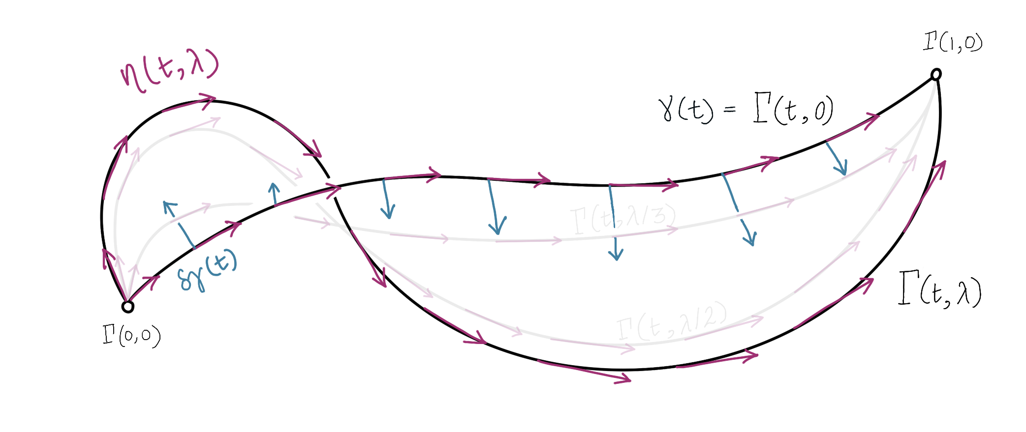

For each $t\in[0, 1]$, this is nothing but a tangent vector of $\mathcal Q$:

\[ \frac{\partial}{\partial\lambda} \Gamma (t, \lambda)\Big\rvert_{\lambda=0} \in T_{\gamma(t)}\mathcal Q. \]

Thus, as we vary $t$, we obtain a vector field along $\gamma$.

An element $\delta\hspace{-1.5pt}\gamma$$\hspace{1pt}\in T_{\gamma} \mathcal P \mathcal Q$ of this tangent space is commonly referred to as a variation of $\gamma$.² It is both a vector in $T_{\gamma} \mathcal P \mathcal Q$ and a vector field (along $\gamma$) on $\mathcal Q$. Since it’s a vector field, we know that $\delta\hspace{-1.5pt}\gamma$ can be expressed as

\[ \delta\hspace{-1.5pt}\gamma(t) \coloneq \frac{\partial}{\partial \lambda} \Gamma(t, \lambda)\Big\rvert_{\lambda=0} =\xi^i(t) \overline E_{i,\gamma(t)}. \]

Meanwhile, the $t$-derivative of $\Gamma$ also defines a vector field:

$$ \dot\Gamma(s,\lambda) \coloneq \frac{\partial}{\partial t} \Gamma(t, \lambda)\Big\rvert_{t=s} = \eta^i(s, \lambda)\overline E_{i,\Gamma(s,\lambda)}.$$

Since $\Gamma(\hspace{1pt}\cdot\hspace{1pt},\lambda)$ coincides with $\gamma$ at $\lambda=0$, we have the compatibility condition $\eta^i(t,0)=\eta^i(t)$.

Notation	Meaning
$\Gamma(\cdot, \lambda)$	perturbed version of $\gamma$
$\delta\hspace{-1.5pt}\gamma$	direction in which $\gamma$ is perturbed (i.e., variation of $\gamma$)
$\dot\Gamma(\cdot, \lambda)$	velocity vector field of $\Gamma(\cdot, \lambda)$
$\left\lbrace \xi^i,\eta^i \right\rbrace_{i=1}^r$	coefficients of $\delta\hspace{-1.5pt}\gamma$ and $\dot\Gamma$, respectively
$\dot{\square}$, $\delta\hspace{0pt}\square$	derivatives of $\square$ with respect to $t$ and $\lambda$, resp.

Now for the tricky part – any variation of $\gamma$ induces a variation of $\dot\gamma$, which can be described by the functions $\lbrace\delta\hspace{-1.5pt}\eta^i\rbrace_{i=1}^r$ defined as follows:

$$ \begin{align*} \delta\hspace{-1.5pt}\eta^i &\coloneq \frac{\partial}{\partial\lambda} \eta^i(s, \lambda)\Big\rvert_{\lambda=0}. \end{align*} $$

As the variational principle requires us to pass from the $n$-dimensional space $\mathcal Q$ to the $(n+r)$-dimensional space $\mathcal Q \times \mathfrak g$, we need additional constraints that relate $\delta\hspace{-1.5pt}\gamma$ to $\lbrace\delta\hspace{-1.5pt}\eta^i\rbrace_{i=1}^r$, ensuring that the variations of $\gamma$ and $\dot \gamma$ are compatible.³ To put it differently, notice that since $\delta\hspace{-1.5pt}\gamma$ determines the perturbed curve $\Gamma(\hspace{1pt}\cdot\hspace{1pt}, \lambda)$ for vanishingly small values of $\lambda$, the value of the velocity vectors are already specified by $\delta\hspace{-1.5pt}\gamma$, meaning that we don’t have the freedom to also specify $\lbrace\delta\hspace{-1.5pt}\eta^i\rbrace_{i=1}^r$ arbitrarily.

Annoyingly, Poincaré considers this matter a triviality. His (translated) paper reads “… and [one] can easily find…” before the result is presented. It is indeed a triviality when $G$ is abelian⁴, in which case we can use what Marsden & Ratiu like to call the equality of mixed partials: $\frac{\partial^2}{\partial t \partial \lambda} = \frac{\partial^2}{\partial \lambda \partial t}$. Much of what follows is a discussion of how this equality manifests in the non-abelian case, without resorting to the convenience of matrix Lie groups.

⌁ Variation of $\dot\gamma$

The reader may want to specialize to matrix Lie groups and finish the argument algebraically, as done in Theorem 13.5.3 of Introduction to Mechanics and Symmetry by Marsden & Ratiu. Here, I will do a slightly more general version of the proof. What follows can be supplemented with Lee’s Introduction to Riemannian Manifolds (Lee IRM).

Consider an affine torsion-free connection $\nabla$ on $\mathcal Q$. The curve $\gamma(t)$ and the connection $\nabla$ together define the covariant derivative operator, $D_t(\hspace{1pt}\cdot\hspace{1pt})$. Using the Symmetry Lemma [Lemma 6.2, Lee IRM], we have

$$ \begin{align*} D_t\left[\frac{\partial}{\partial \lambda}\Gamma(t, \lambda)\Big|_{\lambda=0}\right](s) = D_{\lambda} \left[\frac{\partial}{\partial t}\Gamma(t, \lambda)\Big|_{t=s}\right](0). \end{align*} $$

Either side of this equation is a vector at $\Gamma(s,0)$. The idea is that we need to relate the left-hand side to $\dot\xi^i$ and the right-hand side to $\delta\hspace{-1.5pt}\eta^i$. The left-hand side is⁵

$$ \begin{align*} D_t\delta\hspace{-1.5pt}\gamma(s) &= \dot\xi^i(s)\overline E_{i,\gamma(s)} + \xi^i(s)\big[\nabla_{\dot\gamma(s)}\overline E_{i}\big]_{\gamma(s)}\\ &= \dot\xi^i(s)\overline E_{i,\gamma(s)} + \xi^i(s)\eta^j(s)\big[\nabla_{\overline E_{j}}\overline E_{i}\big]_{\gamma(s)}, \end{align*} $$

whereas the right-hand side is

$$ \begin{align*} D_{\lambda} &\left[\eta^i(s, \lambda)\overline E_{i,\Gamma(s,\lambda)}\right](0) \\&= \frac{\partial }{\partial\lambda} \eta^i(s, \lambda)\Big|_{\lambda=0}\overline E_{i,\Gamma(s,0)} + \eta^i(s, 0) \big[\nabla_{\delta\hspace{-1.5pt}\gamma(s)}\overline E_{i}\big]_{\gamma(s)} \\&= \delta\hspace{-1.5pt}\eta^i(s)\overline E_{i,\gamma(s)} + \eta^i(s)\big[\nabla_{\delta\hspace{-1.5pt}\gamma(s)}\overline E_{i}\big]_{\gamma(s)}\\&= \delta\hspace{-1.5pt}\eta^i(s)\overline E_{i,\gamma(s)} + \xi^j(s)\eta^i(s)\big[\nabla_{\overline E_{j}}\overline E_{i}\big]_{\gamma(s)} \\&= \delta\hspace{-1.5pt}\eta^i(s)\overline E_{i,\gamma(s)} \\&\qquad+ \xi^j(s)\eta^i(s)\hspace{2pt}\big(\hspace{1pt}\nabla_{\overline E_{i}}\overline E_{j} - [{\overline E_{i}}, \overline E_{j} ]\big)_{\gamma(s)}. \end{align*} $$

The last equality (as well as the symmetry lemma itself) follows from the connection being torsion-free. Note that $[{\overline E_{i}}, \overline E_{j} ] = L_{\overline E_{i}} \overline E_{j}$ is the Lie derivative; we will return to this point shortly. For now, we observe that the symmetry lemma yields

$$ \begin{align*} \dot\xi^i(s)\overline E_{i,\gamma(s)} &= \delta\hspace{-1.5pt}\eta^i(s)\overline E_{i,\gamma(s)} - \eta^i(s)\xi^j(s)[{\overline E_{i,\gamma(s)}}, \overline E_{j,\gamma(s)} ]. \end{align*} $$

⌁ Returning to $\mathfrak g$

We are not quite done; the reader will notice that our expression appears to agree with Marsden and Ratiu’s, but has a sign-difference when compared to Poincaré’s. Actually, our equations are closer to Poincaré’s. The apparent discrepancy is due to the fact that the vector fields $\lbrace \overline E_i\rbrace_{i=1}^r$ are more closely related to the right-invariant vector fields (RIVFs) on $G$ than they are to the left-invariant vector fields (LIVFs). In particular, there is a Lie algebra anti-homomorphism: $[{\overline E_i, \overline E_j}] = -\overline{[ E_i, E_j]}$ (proven in the appendix), since the usual Lie bracket on $\mathfrak g$ is also defined via LIVFs. Our urge to make everything “act from the left” in mathematical notation has led us to consider left group actions on $\mathcal Q$, and I suppose the same urge has made LIVFs the predominant choice on $G$.

Let $\xi(s) \coloneq \xi^i(s) E_i$ and $\delta\hspace{-1.5pt}\eta(s) \coloneq \delta\hspace{-1.5pt}\eta^i(s) E_i$ be curves in $\mathfrak g$. Note that $\overline{\small\dot\xi(s)} = \dot\xi^i(s)\overline E_{i,\gamma(s)}$. We have,

$$ \begin{align*} \overline{\small\dot\xi} = \overline{\delta\hspace{-1.5pt}\eta}- \big[\hspace{2pt}\overline{\small {\delta\hspace{-1.5pt}\eta}}\hspace{0.5pt},\hspace{1pt}&\overline{\small \xi}\hspace{2pt}\big]= \overline{\delta\hspace{-1.5pt}\eta} + \overline{[\hspace{1.5pt}{\small\delta\hspace{-1.5pt}\eta}\hspace{0.5pt},\hspace{1pt} {\small \xi\hspace{1.5pt}}]}\\ &\Downarrow \\ \dot\xi={\delta\hspace{-1.5pt}\eta} &+ {[\hspace{1.5pt}{\small\delta\hspace{-1.5pt}\eta}\hspace{0.5pt},\hspace{1pt} {\small \xi\hspace{1.5pt}}]}. \end{align*} $$

Finally, we have something that agrees with Poincaré’s note.[^alt] It agrees with Marsden & Ratiu’s too, but corresponds to the right-invariant version of their result, which in their book is left as an exercise to the reader. In the proof presented by M & R, they consider the right group action of $G$ on $\mathcal Q$, whereas we have considered a left action. Consequently, M & R describe $\dot\Gamma$ and $\delta\hspace{-1.5pt}\gamma$ using their left-invariant velocities, while we had to work with their right-invariant counterparts.

In the basis we chose for $\mathfrak g$, we can compute the structure constants $\lbrace c_{ij}^k\rbrace_{i,j,k=1}^r$, after which we can write

$$ \dot\xi^i = {\delta\hspace{-1.5pt}\eta}^i \ +\ {\delta\hspace{-1.5pt}\eta}^{\hspace{0.5pt}j}\, \xi^k \,c_{jk}^i. $$

Euler-Poincaré Equations

Let $\mathscr L:T\mathcal Q \rightarrow \mathbb R$ be a smooth function, called the Lagrangian (recall that a Hamiltonian $\mathscr H$ is instead a function on $T^\ast \mathcal Q$). Let $\eta(t)\coloneq \eta^i(t)E_i$. Given a tuple $(\gamma(t),\eta(t))$, we can map it to a unique point in $T\mathcal Q$:

$$ (\gamma(t),\eta(t))\mapsto\big(\gamma(t),\overline{\eta(t)}_{\gamma(t)}\big) $$

(this is not precisely the pushforward map of $\Phi$, but it’s very close!) Consequently, we can pull back $\mathscr L$ to define a function on $\mathcal Q \times \mathfrak g$, denoted as $\mathscr L'$. The function $\mathscr L'$ will be invariant under the transformations of $\eta$ that leave $\overline{\eta}$ unchanged.

Now, $\mathscr L'$ can be further pulled back under $\tilde \gamma : t\mapsto(\gamma(t),\eta(t))$ to define $\mathscr L' \circ \tilde\gamma$, a function on $[0,1]$ that can be integrated! Consider the mapping $\mathscr A:\mathcal P(\mathcal Q\times \mathfrak g) \rightarrow \mathbb R$ defined by

$$ \begin{align} \mathscr A(\tilde\gamma) &= \int_0^1 \mathscr L' \circ \tilde\gamma\,(t)\hspace{1pt} dt = \int_0^1 \mathscr L'\big(\gamma(t), \eta(t)\big)\hspace{1pt} dt, \end{align} $$

called the action functional.⁶ Even before we consider the variation in $\gamma$, we already see that $\gamma(t)$ and $\eta(t)$ should satisfy a constraint, namely that $\dot\gamma(t)=\eta^i(t)\overline{E_i}_{\gamma(t)}$. In the classical derivation, this was replaced by the “identity” $\dot q(t) = \frac{d}{dt} q(t)$.

$$ \require{amscd} \begin{CD} \mathcal Q \times \mathfrak g @>{(p,\, X) \mapsto (p,\,\overline{X}_p)}>> T\mathcal Q \\ @A{\tilde\gamma}AA @VV{\mathscr L}V \\ [0,1] @>{{\mathscr L}'\circ\tilde\gamma}>> \mathbb{R} \end{CD} $$

The variations in $\gamma$ and $\eta$, will introduce another constraint. That is, $\delta\hspace{-1pt}\eta$ should be compatible with $\delta\hspace{-1pt}\gamma$ (as was made precise in the preceding section). These variations will together induce a variation in $\mathscr L'$, and consequently in $\mathscr A$, the last of which we will set to $0$. I will write this using coordinates (see Appendix A) because (i) we can, and (ii) I don’t know how to do this in a coordinate-free way (yet):

$$ \begin{align} {d\mathscr A}_\gamma \big((\delta\hspace{-1pt}\gamma, \delta\hspace{-1.5pt}\eta)\big) &= \int_0^1 \left[\frac{\partial \mathscr L'}{\partial\,\gamma^i\,}\delta\hspace{-1pt}\gamma^i + \frac{\partial \mathscr L'}{\partial\,\eta^i\,}\delta\hspace{-1pt}\eta^i\right]\big(\tilde\gamma(t)\big)\hspace{1pt} dt =0. \end{align} $$

The object ${d\mathscr A}_\gamma $ is written by Marsden & Ratiu as $\frac{\delta \mathscr A}{\delta \gamma\ }$ – it is the exterior derivative of $\mathscr A$. Using the compatibility condition from the previous section (as well as App. A), we have

$$ \begin{align} &\int_0^1 \left[\frac{\partial \mathscr L'}{\partial\,\gamma^i\,}\xi^j \overline E_j^i + \frac{\partial \mathscr L'}{\partial\,\eta^j\,}\dot\xi^j \ +\ \frac{\partial \mathscr L'}{\partial\,\eta^i\,}{\delta\hspace{-1.5pt}\eta}^{k} \xi^j c_{jk}^i\right]\hspace{1pt} dt,\\ &=\int_0^1 \xi^j \left[\frac{\partial \mathscr L'}{\partial\,\gamma^i\,} \overline E_j^i - \frac{d}{dt}\left(\frac{\partial \mathscr L'}{\partial\,\eta^j\,}\right)+ \frac{\partial \mathscr L'}{\partial\,\eta^i\,} {\delta\hspace{-1.5pt}\eta}^{k}c_{jk}^i\right]\hspace{1pt} dt\\ &\qquad\qquad\qquad +\int_0^1 \frac{d}{dt}\left(\frac{\partial \mathscr L'}{\partial\,\eta^j\,} \xi^j\right) dt =0. \end{align} $$

But the fundamental theorem of calculus tells us that

$$ \int_0^1 \frac{d}{dt}\left(\frac{\partial \mathscr L'}{\partial\,\eta^j\,} \xi^j\right) dt = \left[\frac{\partial \mathscr L'}{\partial\,\eta^j\,} \xi^j\right]_{t=0}^{t=1}. $$

For variations that fix the endpoints (I explain in the footnotes why we need this constraint), the above term is $0$, and we can localize the integral to obtain the Euler-Lagrange equations:

$$ \begin{align} \frac{d}{dt}\left(\frac{\partial \mathscr L'}{\partial\,\eta^j\,}\right) = \frac{\partial \mathscr L'}{\partial\,\eta^i\,} {\delta\hspace{-1.5pt}\eta}^{k}c_{jk}^i + \frac{\partial \mathscr L'}{\partial\,\gamma^i\,} \overline E_j^i . \end{align} $$

And there it is, une forme nouvelle des équations de la mécanique. As Poincaré points out, this is especially of interest when $\mathscr L'$ only depends on $\eta$ (e.g., when computing geodesic motion).

---

Appendices

A. Computation in Coordinates

Let $\lbrace q^i\rbrace_{i=1}^n$ be coordinates on a subset of $\mathcal Q$. We can express $\overline E_i$ in terms of the coordinate frame $\lbrace {\partial}/{\partial q^i}\rbrace_{i=1}^n$, as

$$\overline E_i = \overline E_i^j \frac{\partial}{\partial q^j},$$

where each $\overline E_i^j \in C^\infty(\mathcal Q)$ is a coordinate function. Letting $\overline E_i$ act on the coordinate function $q^j$, we get

$$ \overline E_i q^j = \overline E_i^k \frac{\partial q^j}{\partial q^k} = \overline E_i^j, $$

which tells us how to compute the coefficients of $\overline E_i$ – just feed it the coordinate functions. Returning to the definition of $\dot\gamma(s)$, we get:

$$\dot\gamma(s) = \eta^i(s) \overline E_i^j(\gamma(s)) \frac{\partial}{\partial q^j}\Big\vert_{\gamma(s)}.$$

Letting the left-hand side act on the coordinate function $q^k$, we get

$$ \begin{align*} \big(\dot\gamma(s)\big) (q^k) &= d \gamma_s \left(\frac{\partial}{\partial t}\Big\rvert_{t=s}\right)(q^k)=\frac{d}{dt}(q^k\circ \gamma)(t)\Big|_{t=s}, \end{align*} $$

whereas letting the right-hand side eat $q^k$, we get

$$ \begin{align*} \eta^i(s) \overline E_i^j(\gamma(s)) \frac{\partial q^k}{\partial q^j}\Big\vert_{\gamma(s)} = \eta^i(s) \overline E_i^k(\gamma(s)). \end{align*} $$

Here, $i$ sums from $1$ to $r$ whereas $j$ sums (and $k$ ranges) from $1$ to $n$. Also, observe that $r\geq n$ due to transitivity of the group action. Denoting $q^j \circ \gamma$ as $\gamma^j$, we can finally put everything together:

$$ \frac{d \gamma^k}{dt}(s) = \eta^i(s) \overline E_{i,\gamma(s)} \gamma^k(s). $$

This expression can be found in Poincaré’s paper (linked at the beginning of the post). Similarly, we have

$$ \begin{align*} \delta\hspace{-1.5pt}\gamma(s) =\delta\hspace{-1.5pt}\gamma^i(s)\frac{\partial}{\partial q^i}\Big\vert_{\gamma(s)} = \xi^j(s) \overline E_j^i \frac{\partial}{\partial q^i}\Big\vert_{\gamma(s)}. \end{align*} $$

B. Computation using Matrix Algebra

We can choose $\Gamma$ to be

$$\Gamma(t, \lambda) = \exp(\lambda \xi^i(t) E_i)\cdot\gamma(t)$$

since it satisfies the conditions for being a representative of $\delta\hspace{-1.5pt}\gamma$. Actually, we can do something more; we can express $\gamma(t)$ as $g(t) \cdot p$, where $p\in \mathcal Q$ is a some distinguished point (that may be called the “origin” of $\mathcal Q$) and $g(t)$ is a curve of actions in $G$. This means that

$$\Gamma(t, \lambda) = \exp(\lambda \xi^i(t) E_i)g(t)\cdot p.$$

The curve $g$ that generates $\gamma$ in this manner is not unique even after we have fixed some point $p$. To see why, one can consider (the rather silly example of) $G=\mathbb R^3 \times \mathbb R^3$ and $\mathcal Q = \mathbb R^3$. Nevertheless, since we are going to probe all possible variations of $\gamma$, we only need to worry about the “surjectivity” of this formulation, rather than its “injectivity”. Surjectivity follows from our assumption of the group action being transitive.

If $G$ is a matrix Lie group, the expression

\[ \begin{align*} \frac{d}{d t}&\left(\left( \frac{\partial}{\partial \lambda} \Gamma(t, \lambda)\Big\rvert_{\lambda=0}\right)g(t)^{-1}\right) \end{align*} \]

can be viewed from a purely matrix-algebraic lens. This is what Marsden and Ratiu do in their book, so I leave the remaining details to them.

C. Proof of $[{\overline X, \overline Y}] = -\overline{[ X, Y]}$

Let $\bar L^{(g)} (q) \coloneq \Phi(g,q) = \Phi^{(q)}(g)= g\cdot q$. We will reuse this notation for left and right multiplication on $G$, so that $L^{(g)}(h)=R^{(h)}(g) = gh$. The following equalities hold:

$$ \begin{align*} g\cdot(h\cdot q)&=gh\cdot q\\ \quad\bar L^{(g)}\circ \bar L^{(h)} &= \bar L^{(gh)}\\ \bar L^{(g)} \circ \Phi^{(q)} &= \Phi^{(q)}\circ L^{(g)}\ \ \\ \Phi^{(h\cdot q)} &= \Phi^{(q)}\circ R^{(h)} \end{align*} $$

As a mnemonic, we can think of $\Phi^{(q)}$ as “right-multiplication by $q$”, so that it “commutes” with $\bar L^{(g)}$. Next, we need to demonstrate the fact that $\overline{\mathrm{Ad}_g Y}={\bar L^{(g^{-1})}}^\ast\hspace{1pt} \overline Y$. The vector field on the left has, at $q\in\mathcal Q$, the value

$$ \begin{align*} d\Phi^{(q)}_e (\mathrm{Ad}_g Y) &= d\Phi^{(q)}_e dR^{(g^{-1})}_{g} dL^{(g)}_e Y\\ &= d\Phi^{(g^{-1}\cdot \hspace{1pt}q)}_{g} dL^{(g)}_e Y. \end{align*} $$

The corresponding vector on the right is

$$ ({L^{(g^{-1})}}^\ast\hspace{1pt} \overline Y)_q = (L^{(g)}_\ast\hspace{1pt} \overline Y)_q = {(d \bar L_{g})}_{g^{-1}\cdot \hspace{1pt}q} d\Phi_{e}^{(g^{-1} \cdot\hspace{1pt} q)} Y, $$

and the “commutativity” of $\bar L^{(g)}$ and $\Phi^{(q)}$ completes the argument.

Next, choose $g=\exp(tX)$ and differentiate w.r.t $t$ (i.e., evaluate the pushforward of $\frac{\partial}{\partial t}$):

$$ \begin{align*} \overline{\frac{d}{dt}\mathrm{Ad}_{\exp(t X)} Y\Big\rvert_{t=0}} &= \frac{d}{dt} {\bar L^{(\exp(-tX))}}^\ast \overline Y\Big\rvert_{t=0}\\ \overline{\mathrm{ad}_X Y} &= -\frac{d}{dt} {\bar L^{(\exp(tX))}}^\ast \overline Y\Big\rvert_{t=0}\\ \overline{[X,Y]} &= -[\overline{X}, \overline{Y}]. \end{align*} $$

The last line follows from the fact that $\bar L^{(\exp(tX))}$ is the flow of $\overline{X}$, and that the Lie bracket of vector fields is (by definition) the Lie derivative.