Let $\mathcal X$ be a Hilbert space, which means that it is a vector space that has an inner product (denoted by $\langle \cdot, \cdot\rangle _\mathcal X$) and that it is complete, i.e., it doesn’t have er… holes in it. Recall that inner product spaces have a rich geometric structure, and so do Hilbert spaces. The Euclidean space $\mathbb R^n$ is an obvious example, where the inner product is just the dot product. Mathematicians sometimes use ‘Hilbert space’ to refer specifically to infinite-dimensional inner product spaces, but for our purposes, we will let ‘Hilbert space’ include the finite-dimensional case.
Some interesting Hilbert spaces are given below. Each of these spaces has a corresponding norm, $\lVert x \rVert_{\mathcal X}=\sqrt{\langle x, x\rangle}_{\mathcal X}$, which we call as the norm that is induced by the inner product.
| Hilbert Space $\mathcal X$ | Inner Product $\langle \cdot, \cdot\rangle _\mathcal X$ |
|---|---|
| Numbers $a$, $b\in \mathbb R$ | $ab$ |
| Random Variables $X,Y\in \mathbb R$ | $\mathbb E \left[XY \right]$ |
| Real Vectors $x$, $y\in \mathbb R^n$ | $\mathbf x^\intercal \mathbf y$ |
| Complex Vectors $x$, $y\in \mathbb C^n$ | $\mathbf x^\dagger \mathbf y$ |
| Matrices $\mathbf A$, $\mathbf B\in \mathbb R^{m\times n}$ | $\ \text{Trace}(\mathbf A^{\intercal}\mathbf B)$ |
| Sequences $(x_i)_{i=1}^{\infty}, (y_i)_{i=1}^{\infty}\in \ell ^2(\mathbb R) \ $ | $\sum_{i=1}^{\infty} x_i y_i$ |
| Square-Integrable Functions $f,g \in L^2(\mathbb R)$ | $\int_{-\infty}^{\infty}f(x)\overline{g(x)}dx$ |
Here, $\overline{({}\cdot{})}$ is the conjugate of a complex number (where you replace $i$ with $-i$), $({}\cdot{})^\dagger =\overline{({}\cdot{})}^\intercal $ is called the conjugate transpose of a complex vector.
Projections
A defining feature of Hilbert Spaces is their geometry. Because they have notions of angles , we have
$$ 0 \leq {|\langle x, y\rangle_{\mathcal X} |} \leq {\|x\|\|y\|} $$where if the first equality holds we say $x$ and $y$ are orthogonal to each other, and the second equality holds if and only if they are linearly dependent: $x = a y$ for $a \in \mathbb R$ (or $\mathbb C$, when $\mathcal X$ is a complex vector space).
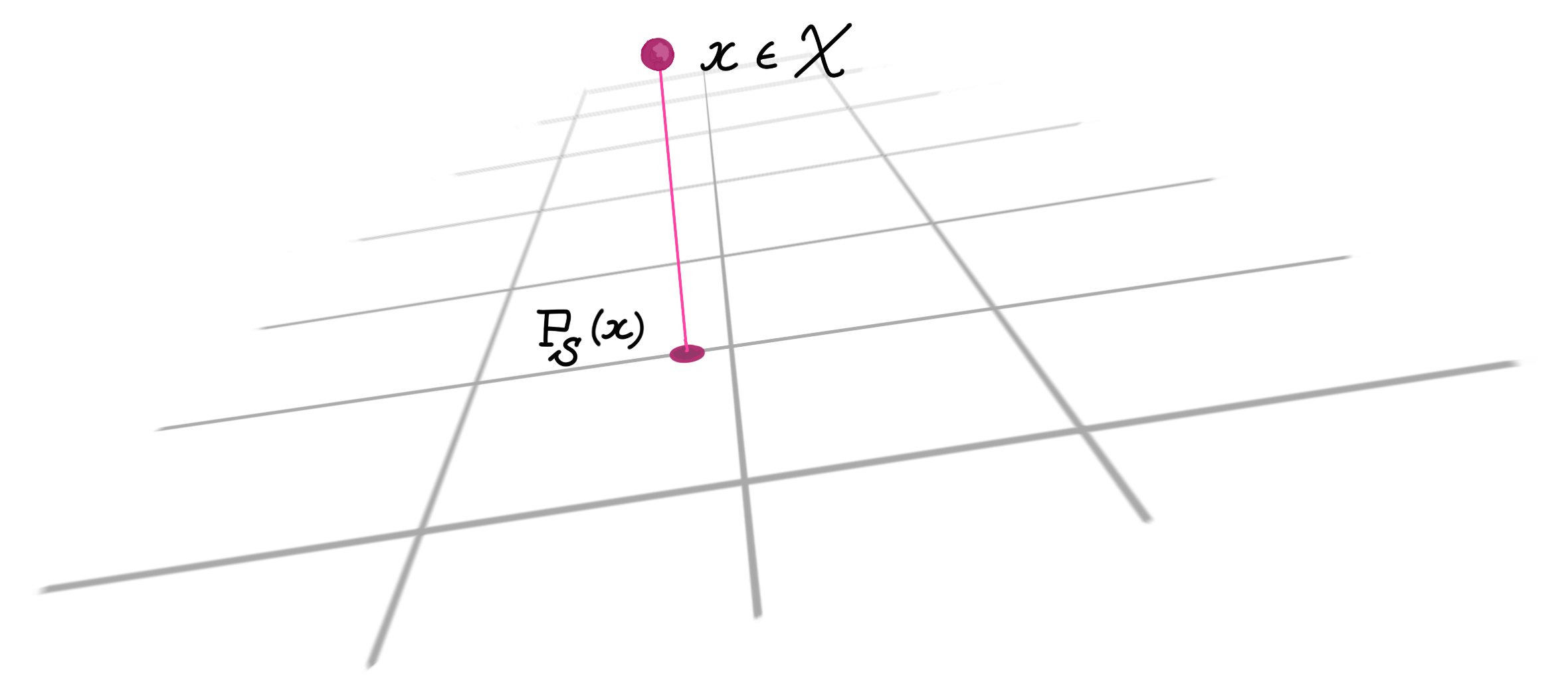
We can define the projection of an element $x\in \mathcal X$ onto a subspace $S\subseteq \mathcal X$:
\[ \text{P}_S(x) = \mathrm{argmin}_{y\in S}\|x-y\|_{\mathcal X}\]
where $\lVert v \rVert_{\mathcal X} = \sqrt{\langle v, v\rangle}_{\mathcal X}$ is the induced norm. A remarkable by-product of these definitions of angles, orthogonality, and projection, is that it is consistent with our Euclidean intuition: $x-\text{P}_S(x)$ is always orthogonal to $S$. A related theorem says that $\text P_{\tilde S}(x)$ is well-defined and unique even if $\tilde S \subseteq \mathcal X$ is a closed convex set, although in this case we do not have orthogonality of $x-\text{P}_{\tilde S}(x)$ to the other elements in $\tilde S$.
As an example, given two ‘vectors’ $X$ and $Y$ in the Hilbert space of random variables, orthogonality corresponds to $\mathbb E\left[X Y\right] = 0$ and the norm becomes the variance. In this case, orthogonal projection actually gives the least-squares estimator of given a random variable ( Lec. 22, p. 85 ). More generally, a projection can be used to compute the best approximation of an element of a Hilbert space (namely, the point being projected), with the approximation constrained to lie on a subspace (or a closed convex set).
The $(\mathbb R^N, \lVert{}\cdot{}\rVert_2)$ Space of Sequences
Given a vector in the Euclidean space $\mathbb R^N$ (equipped with a basis), we can view it as a set of $N$ coefficients. Each coefficient (a real number) describes the vector’s distance along the corresponding basis vector (or ‘axis’, if you will).
Taking a few steps back, let’s begin by viewing $\mathbb R^N$ as the set-theoretic product $\mathbb R \times \mathbb R \times \dots \times \mathbb R$. An element $x$ of this space is a sequence of real numbers,
\[x = (x_1, x_2, \dots, x_N).\]
Once we define notions of addition and scalar multiplication for such $N$-coefficient sequences, we are allowed to call $\mathbb R^N$ a vector space. A norm for $\mathbb R^N$ can be defined as $\left(\sum_{i=1}^N |x_i|^2\right)^{1/2}$, which automatically induces a topology (notion of open and closed sets) on $\mathbb R^N$. We can generalize all of this as $N\rightarrow \infty$.
The $\ell^2$ Space of Sequences
$\ell^2(\mathbb R)$ consists of countable sequences of real numbers. ‘Countable’ here means that we can count them like we can count the natural numbers, but they are infinitely long nonetheless. We denote one such sequence as $(x_i)_{i=1}^{\infty}$. A sequence is in $\ell^2$ if and only if it is square-summable, which means
\[ \sum_{i=1}^{\infty}|x_i|^2 < \infty \]
A sequence which is not in $\ell^2$ (i.e., an ‘infinite-length vector’) is $\left(\frac{1}{\sqrt{1}}, \frac{1}{\sqrt{2}}, \frac{1}{\sqrt{3}}, \dots\right)$ because its sum-of-squares decays too slowly as the number of terms increases. A sequence that is in $\ell ^2$ is $\left(\frac{1}{1}, \frac{1}{2}, \frac{1}{3}, \dots\right)$.
(Separable) Hilbert Spaces are Isomorphic
Isomorphisms are maps from one type of mathematical object to another that preserve its structure. All (separable) infinite-dimensional Hilbert spaces are isomorphic to the $\ell^2$ space , which is a fancy way of saying that we can do the following: We first construct a countable orthonormal basis for $\mathcal X$ (e.g., using the Gram-Schmidt process and perhaps Zorn’s lemma ), denoted as $(e_i)_{i=1}^{\infty}$. Then, we define an isometric isomorphism (a distance-preserving, structure-preserving mapping) from $\mathcal X$ to $\ell^2$, as follows:
\[T: \mathcal X \rightarrow \ell^2\] \[T(x) = (\langle e_i,x \rangle_{\mathcal X})_{i=1}^{\infty} \]
which is the sequence of coefficients of $x$ along each basis vector. Note that $T$ is basis-dependent, we could pick a different basis and get a different $T$. Since $T$ is an isomorphism (i.e., does not ‘destroy’ information during the mapping), we may hope to be able to go back from $\ell^2$ to $\mathcal X$:
\[T^*: \ell^2 \rightarrow \mathcal X\] \[T^{*}\left((c_i)_{i=1}^{\infty}\right) = \sum_{i=1}^{\infty} c_i e_i \]
Here, $T^{*}$ is called the adjoint of $T$; it is an operator that satisfies
\[\langle y,T(x)\rangle _{\ell^2} = \langle T^*(y),x\rangle _{\mathcal X}\]
The map $T({}\cdot{})$ is necessarily linear , and it can be shown that $T^*$ is the inverse of $T$ (i.e., $T^\ast = T^{-1}$, something which is not true for general linear transformations!). The mapping $T({}\cdot{})$ can be represented via a matrix, although this matrix has infinitely many rows and columns.
Using a similar reasoning as above in the finite-dimensional case, we see that all (separable) complex Hilbert spaces with dimension $N$ are isomorphic to the $(\mathbb C^N, \lVert{}\cdot{}\rVert_2)$ space. The condition that $T^*=T^{-1}$ might remind you of unitary matrices ($U^\dagger = U^{-1}$, where $U^\dagger$ is the conjugate transpose of $U$), which are exactly the distance-preserving, structure-preserving matrices in $\mathbb C^N$. When we’re working with real Hilbert spaces we replace $\mathbb C^N$ with $\mathbb R^N$ and ‘unitary’ with ‘orthogonal’. Recall that $Q^\intercal = Q^{-1}$ for an orthogonal matrix $Q$. Orthogonal matrices are an isometry (distance-preserving) because $\lVert Qx\rVert_2 = \lVert x \rVert_2$, and they are an isomorphism (structure-preserving) because $\langle Qx, Qy \rangle =\langle x, Q^\intercal Qy \rangle = \langle x, y\rangle$. Note that isomorphisms also preserve the angles between vectors.
The $L^p$ Space of Functions
Let’s move onwards to function spaces. The space $L^1(\mathbb R)$ is the space of absolutely integrable functions. An element $f\in L^1(\mathbb R)$ is a function of the form $f:\mathbb R\rightarrow \mathbb C$ and satisfies
$$ \| f\|_{L^1} =\int_{\mathbb R} | f(x)| dx < \infty.$$It is clear how to add and (pointwise) multiply functions, so $L^1(\mathbb R)$ is indeed a vector space. The space $L^2(\mathbb R)$ consists of functions which are square-integrable:
$$ \| f\|_{L^2} =\left(\int_{\mathbb R} | f(x)|^2dx\right)^{1/2} < \infty$$and is a Hilbert space because it has the following inner product + norm combination:
$$ \begin{align} \langle f, g \rangle_{L^2} &= \int_{\mathbb R} f(x) \overline{g(x)} dx\\ \| f\|_{L^2} &= \sqrt{ \langle f, f \rangle_{L^2}}. \end{align}$$Can we use the above as an inner product for $L^1$ as well? It turns out that we can’t, because even if $f$ is in $L^1$, the integral of $f(x)\overline{f(x)}$ can be unbounded if $f$ is not also in $L^2$.
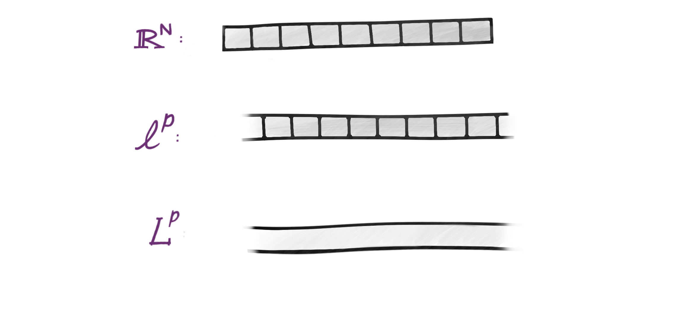
The norms on $\ell^p$ and $L^p$ spaces are natural extensions of the $p$-norms for finite-dimensional vector spaces, and as expected, we have an inner product only when $p=2$. The $L^p(\mathbb R)$ space can be thought of as a ‘refinement’ of the domain of the $\ell^p$ space1, where the index set $\lbrace 1, 2, \dots, \infty\rbrace$ (which was countable) of $\ell^p$ is replaced with $\mathbb R$ (which is uncountable) in $L^p$. So even though these might seem like completely different concepts thrown together, they are closely related and inherit much of each other’s properties!
But since $L^2$ and $\ell^2$ are supposed to be isomorphic, this suggests that we can go from $L^2$ to $\ell^2$ (and back) using a linear map. The fact that we can represent an arbitrary function on a continuous domain using a sequence of numbers is remarkable.
Fourier Transforms
This section is for people who might have encountered the Fourier transform before, and want to see the Hilbert space interpretation of it. Consider a function $f\in L^2([0,1])$, such that $f(t)$ represents the amplitude of a signal at time $t$. The sinusoid is one such signal: $f(t)=\sin (t)$. An orthogonal basis for $L^2([0, 1])$ is $(e_k)_{k\in \mathbb Z}$, where
$$e_k(t)=\frac{1}{\sqrt{2 \pi}}e^{2 \pi i k{t}}.$$Here, $\mathbb Z$ are the integers, which is still a countable set because we can count them as $(0, 1, -1, 2, -2, \dots)$. In this case, our isomorphism $T$ from $L^2([0,1])$ to $\ell^2$ is given by:
$$\begin{align} T(f) &= \left(\langle f, e_k \rangle \right)_{k\in \mathbb Z}\\ &= \left( \frac{1}{\sqrt{2\pi}}\int_{0}^1 f(t)e^{-2\pi i kt} dt\right)_{k\in \mathbb Z} \end{align}$$These are exactly the Fourier coefficients (up to a constant factor, depending on how you define them)! Each coefficient tells you how much of a certain frequency is present in a signal. The way we have defined them (with proper normalization of the basis vectors) ensures that the Fourier transform $T$ is an isometric isomorphism. In fact, the observation that
$$\langle f, g\rangle_{L^2([0,1])} = \langle T(f), T(g)\rangle_{\ell^2}$$has a special name in the signal processing community: it’s called Parseval’s (or Plancherel’s) theorem. We can also discard some of the Fourier coefficients to compress (or de-noise) a signal by ignoring its weak (or bothersome) frequencies – be it an audio signal or an image. Such a truncation of the sequence is a special case of the projection operation in Hilbert spaces, so it’s the best approximation in terms of the $L^2$ norm of the approximation error.
One of the motivations for defining the map $T$ is that we can now represent objects in an arbitrary Hilbert space using a (countable) set of numbers (in $\ell^2$). Aside from being a powerful theoretical tool, it lets us store and manipulate these objects on computers efficiently, as evidenced by the example of the Fourier transform.
All that said, the reason I love typing out posts like these is because it’s so gratifying to see all of these different mathematical objects be unified under a single concept. The interplay between vectors, sequences, and functions is something that was never taught or emphasized to me in school. All throughout college, my instructors usually pulled the Fourier transform out of their hat, just to use it for 2 lectures and then put it back in before I ever figured out what it was. Maybe I’m just a slow learner, so it’s a good thing I have (one would hope) a long life ahead of me to keep learning!