A Lie group $G$ is a group that is also a (continuous, differentiable) topological space. An example to keep in mind is $G=\mathbb R^n$ which is a group under vector addition and has well-defined notions of continuity and differentiation. To measure lengths and volumes (and relatedly, to define and integrate probability densities) we need to endow $G$ with additional structure so that it is not merely a manifold, but a Riemannian manifold. Luckily for us, we only need to define an inner product for the Lie algebra, after which there is a natural definition of length and volume that can be made for the entire group manifold. I say that the resulting choice of volume (called the Haar measure) is natural because it is compatible with the group structure of $G$ as well as its differential structure as a manifold. This can be compared to how the standard notion of volume for $\mathbb R^n$, the Lebesgue measure, is compatible with vector addition; we have for a (measurable) set $A\subseteq \mathbb R^n$ and for every $\mathbf x_0 \in \mathbb R^n$,

$$\textrm{Vol}(A) = \textrm{Vol}(\lbrace \mathbf x + \mathbf x_0 \ \vert\ \mathbf x \in A \rbrace).$$

Thus begins our journey into making sense of this compatibility in the general context of a Lie group. If you are seeking a more application-oriented approach and/or aren’t all that interested in this sort of abstraction, this book has all the formulae worked out, and my previous post introduces the idea of invariant metrics and measures on Lie groups. Note that I will be using the Einstein summation convention throughout.

Lengths and Volumes ✨

Let $M$ be an $n$-dimensional smooth manifold. A covariant $2$-tensor field on $M$ is a bilinear map that takes $2$ smooth vector fields as its arguments and produces a smooth $C^\infty(M)$ function.¹ A Riemannian metric is a covariant $2$-tensor field that is symmetric:

$$\begin{align} g(\mathbf{v}_1, \mathbf{v}_2) &= g(\mathbf{v}_2, \mathbf{v}_1) \in C^\infty(M), \end{align}$$

and positive-definite:

$$\begin{align} g(\mathbf{v}_1, \mathbf{v}_1)(p) > 0 &\quad \Leftrightarrow \quad \mathbf{v}_1(p) \neq \mathbf 0. \end{align}$$

where $\mathbf{v}_1, \mathbf{v}_2 \in \mathfrak X(M)$ are smooth vector fields on $M$. At some point $p\in M$, the number $g(\mathbf{v}_1, \mathbf{v}_2)(p)$ is interpreted as the inner product between the tangent vectors $\mathbf{v}_1(p)$ and $\mathbf{v}_2(p)$, often written as $\langle \mathbf v_1, \mathbf v_2 \rangle_p \coloneqq g(\mathbf{v}_1, \mathbf{v}_2)(p)$. With such a mathematical structure imposed on $M$, we call $(M,g)$ a Riemannian manifold.

While a metric tensor is a symmetric covariant $2$-tensor field, a volume form $\omega$ is an alternating covariant $n$-tensor field, also called as a differential $n$-form. By combining its alternating property with its linearity, $\omega$ can be shown to be antisymmetric in its arguments. That is, if $\mathbf{v}_1,\mathbf{v}_2, \cdots, \mathbf{v}_n \in \mathfrak X(M)$ are smooth vector fields, then

$$\omega(\mathbf{v}_1, \mathbf{v}_2, \cdots, \mathbf{v}_n) = -\omega(\mathbf{v}_2, \mathbf{v}_1, \cdots, \mathbf{v}_n) = \nu \in C^\infty(M)$$

The function $\nu$ that is spit out by $\omega$ (after it eats $n$ vector fields) assigns the volume $\nu(p)\in \mathbb R$ to the parallelopiped spanned by the vectors $\mathbf{v}_1(p), \mathbf{v}_2(p), \cdots, \mathbf{v}_n(p)\in T_pM$. Thus, $\omega$ is sort of like a ‘volume meter’ affixed to each point of $M$. It is the authority on what counts as a positive volume, what counts as a small or a large volume, and so on. Its antisymmetry can be compared with the fact that $\int_a^b f(x) dx= -\int_b^a f(x) dx$.

Either of these maps can be written as a tensor in local coordinates on $U\subseteq M$, e.g., $g=g_{ij}dx^i \otimes dx^j$, where the Einstein summation convention is used and $g_{ij}\in C^\infty (U)$. Since the standard tensor notation doesn’t reflect the symmetry/antisymmetry of the tensors, one typically drops it in favor of notation that does:

$$\begin{align} g &= g_{i_1 i_2}dx^{i_1} dx^{i_2}\\ \omega &= \omega_{i_1 i_2 \cdots i_n} dx^{i_1} \wedge dx^{i_2} \wedge \cdots \wedge dx^{i_n} \end{align}$$

This helps us remember that the $dx^{i_1}$ and $dx^{i_2}$ of $g$ can be swapped without consequence, whereas swapping the $dx^{i_1}$ and $dx^{i_k}$ of $\omega$ may or may not incur a sign-change depending on the parity of the permutation.

With this notation, observe that if $\mathbf{v} = v^k \frac{\partial}{\partial x^k}$ and $\mathbf{w} = w^l \frac{\partial}{\partial x^l}$ are vector fields on $U$, where $(\frac{\partial}{\partial x^i})_i$ is the dual basis of $(dx^i)_{i}$, then

$$\begin{align} g(\mathbf{v},\mathbf{w}) &= g_{ij} dx^i dx^j \left(v^k \frac{\partial}{\partial x^k}, w^l \frac{\partial}{\partial x^l}\right) \\ &= g_{ij}v^k w^l \ \left[dx^i dx^j \left(\frac{\partial}{\partial x^k}, \frac{\partial}{\partial x^l}\right)\right] \\ &= g_{ij} v^k w^l \delta^i_k \delta^j_l \\ &= g_{ij} v^i w^j. \end{align}$$

Since it is a (pointwise) sum of (pointwise) products of $C^\infty(U)$ functions, $g_{ij} v^i w^j\in C^\infty(U)$. The metric tensor coefficients $(g_{ij})_{i,j=1}^n$ play a role similar to that of a weighting matrix $W \in \mathbb R^{n \times n}$ that is introduced when defining a non-standard inner product in $\mathbb R^n$, as $\langle \mathbf{v}, \mathbf{w}\rangle \coloneqq \mathbf{v}^\top W \mathbf{w}$.

Frames ✨

In the above expressions, we used a frame (a system of vector fields) that arises from a coordinate chart. However, there may arise situations where we prefer to work with a frame that is not only not induced by a coordinate chart, but also cannot be induced by a coordinate chart. The frame of left-invariant vector fields on a (non-Abelian) Lie group is a prime example of this.

A local frame in an open set $U$ of $M$ is a set of tangent vector fields in $\mathfrak X(U)$, enumerated as $(E_i)_{i=1}^n$, such that $(E_i(p))_{i=1}^{n}$ is a basis of $T_p M$ for all $p\in U\subseteq M$. A local frame is orthonormal if $g(E_i, E_j) = \delta_{ij}$, where $\delta_{ij}$ is the Kronecker delta considered as a constant-valued $C^\infty(U)$ function. A global frame is one that is defined on all of $M$, with $U=M$.

The dual coframe to $(E_i)_{i=1}^n$ is the collection of cotangent (or covariant) vector fields $(\varepsilon^i)_{i=1}^n$, such that $\varepsilon^i(E_j) = \delta^i_{j}$. These cotangent vector fields form a basis for differential $1$-forms. We can take their tensor products to obtain a basis for covariant $k$-tensor fields:

$$\begin{align} \lbrace \varepsilon^{i_1} \otimes \varepsilon^{i_2} \otimes \cdots \otimes \varepsilon^{i_k}\ \vert\ 1\leq i_1, i_2, \cdots, i_k \leq n \rbrace \end{align}$$

or their exterior /wedge products to obtain a basis for the space of differential $k$-forms:

$$\begin{align} \lbrace \varepsilon^{i_1} \wedge \varepsilon^{i_2} \wedge \cdots \wedge \varepsilon^{i_k}\ \vert\ 1\leq i_1 < i_2 < \cdots < i_k \leq n \rbrace \end{align}$$

🍩 Orthonormal Frames

In the coordinate coframe $(dx^i)_{i=1}^n$, we expressed the metric tensor as $g = g_{ij}dx^i dx^j$. Let’s now try to express it in a local coframe $(\varepsilon^i)_{i=1}^n$ on $U \subseteq M$ that is dual to an orthonormal one:

$$\begin{align} g = g_{ij}dx^i dx^j = \tilde g_{ij} \varepsilon^i \varepsilon^j \end{align}$$

We have then, that

$$\begin{align} \delta_{kl} = g(E_k, E_l) &= \tilde g_{ij} {\varepsilon}^i {\varepsilon}^j \left(E_k, E_l\right) \\ &= \tilde g_{ij} {\varepsilon}^i \left(E_k\right) {\varepsilon}^j \left(E_l\right) \\ &= \tilde g_{ij} \delta^i_k \delta^j_l = \tilde g_{kl}. \end{align}$$

This means that the metric tensor, when expressed in a coframe dual to an orthonormal one, has the trivial representation: $g = \delta_{ij} \varepsilon^i \varepsilon^j$. By writing out the summation explicitly, this takes a more familiar form:

$$g = (\varepsilon^1)^2 + (\varepsilon^2)^2 + \cdots + (\varepsilon^n)^2.$$

Given a local orthonormal frame of vector fields $(E_i)_{i=1}^n$ whose dual coframe is $(\varepsilon^i)_{i=1}^n$, the unique (up to choice of orientation) Riemannian volume form $\omega_g$ is given by

$$\begin{align} \omega_g = \varepsilon^1 \wedge \varepsilon^2 \wedge \cdots \wedge \varepsilon^n \end{align}$$

so that $\omega(E_1, E_2, \cdots, E_n) = 1$. The above statements will look identical in any of the local orthonormal frames of $M$.

🍩 Coordinate Frames

The allure of orthonormal frames is that $g$ and $\omega_g$ can be represented quite succinctly in them. However, the existence of an orthonormal frame that arises as the coordinate frame of a chart is a very rare occasion: such a frame only exists when the Riemannian manifold $(M, g)$ is locally flat. If we would rather work with a frame that arises from coordinates, then we must resort to computing the components of a non-flat metric tensor (one that is not simply the Kroenecker delta). Also see my post on the non-flatness of the sphere .

Let $\frac{\partial}{\partial x^i}\Big\vert_{q}$ be the usual coordinate-wise partial derivative operators in $\mathbb R^n$, $q \coloneqq (q_1, q_2, \dots, q_n)$, and $q\in V \subseteq \mathbb R^n$. Given a smooth function $f\in C^\infty(V)$, the partial derivative operators of $\mathbb R^n$ operate on $f$ as follows:

$$\begin{align*} \frac{\partial}{\partial x^2}\bigg\vert_{q} f = \lim_{h\rightarrow 0} \frac{f(q_1, q_2+h, \dots, q_n) - f(q_1, q_2, \dots, q_n)}{h} \end{align*}$$

Recalling that the job of a vector field is to map a smooth function to a real number at every point (in a smooth manner), the following object is in fact a vector field on $V$: $$\frac{\partial}{\partial x^i}\bigg\vert_{(\ \cdot\ )}:V \rightarrow TV.$$ Thus, $\left\lbrace\frac{\partial}{\partial x^i}\big\vert_{(\ \cdot\ )}\right\rbrace_{i=1}^n$ is a set of vector fields on $V$, and may be visualized as a “fisherman’s net” spread across $V$.

Ultimately, we want a coordinate frame on a subset $U$ of $M$, rather than on $V$, which is in $\mathbb R^n$. Let $\varphi:U \rightarrow V$ be a smooth chart containing some point $p$ of $M$. Its differential $(\varphi_*)_p$ is a vector space isomorphism (i.e., an invertible linear map) between $T_p U$ and $T_q V$. The pushforward of the “partial derivative vector fields” of $V$ under $\varphi^{-1}$ gives us a coordinate frame on $U$. That is, $\varphi^{-1}$ maps the fisherman’s on $V$ to one on $U$. By an abuse of notation, I and many others use $\left(\frac{\partial}{\partial x^i}\big\vert_{(\ \cdot\ )}\right)_{i=1}^n$ to refer to either frame; the subscript, the function being operated on, and/or the context will make it clear which frame is being used. This means that if $\tilde f\in C^\infty (U)$, then we write

$$\begin{align} \frac{\partial}{\partial x^i}\Big\vert_{p} \tilde f &= \left((\varphi_*^{-1})_{\varphi(p)} \frac{\partial}{\partial x^i}\Big\vert_{\varphi(p)}\right) \tilde f\\ &= \frac{\partial}{\partial x^i}\Big\vert_{\varphi(p)} \tilde f \circ \varphi^{-1} = \frac{\partial}{\partial x^i}\Big\vert_{\varphi(p)} (\varphi^{-1 *} \tilde f). \end{align}$$

where $\varphi^{-1 *} \tilde f$ is called the pullback of $\tilde f$ under $\varphi^{-1}$; it pulls the domain of $\tilde f$ back to $V$.

🍩 Orthonormal Coordinate Frames

I reiterate that there are Riemannian manifolds where such a coordinate frame couldn’t possibly be orthonormal at all $p\in U$. Theorem 13.14 of Lee’s Introduction to Smooth Manifolds says that this is only possible when $U$ is flat, i.e., $M$ is locally flat.

---

Pullbacks ✨

Let $f:M \rightarrow N$ be a diffeomorphism between manifolds (though it is possible to generalize the forthcoming discussion to other kinds of smooth maps).

Recall that tangent and cotangent vectors are dual to each other, and so are their $k^{th}$ exterior powers: alternating $k$-vector fields and differential $k$-forms. Whenever we have a morphism for an object going one way, we expect a dual morphism for the corresponding dual object going the other way. Using this intuition, we deduce that if $f_*: TM \rightarrow TN$ allows us to push forward vector fields, there must be a dual morphism $f^*: T^* N \rightarrow T^* M$ that allows us to pull back covector fields. Similarly, $f^*: \Omega^k(N) \rightarrow \Omega^k(M)$² pulls back differential forms from $N$ to $M$ (we use the same notation for either map, $f^*$). In particular, metrics and volume forms on $N$ can be pulled back to define metrics and volume forms on $M$.

The covariant tensor field thus obtained on $M$ is called as the pullback of the covariant tensor field on $N$ under $f$. For example, consider $M=S^2$ to be the unit $2$-sphere and $f$ to be its usual submersion into $N=\mathbb R^3$. Then, the pullback of the Euclidean (‘dot product’) metric $\bar g$ of $\mathbb R^3$ under $f$, $f^* \bar g$, is called the round metric, and it is a bonafide Riemannian metric for $S^2$ (I compute its components in the next post ). When the Euclidean metric is pulled back onto a submanifold $M\subseteq \mathbb R^3$ in this manner, the pullback metric is called the induced metric or the first fundamental form of $M$. More generally, we can pull back covariant tensor fields from arbitrary manifolds, as long as we have a smooth map onto it.

The pullback of a differential form is defined such that it must be in concordance with the pushforwards of vector fields. Specifically, if $\omega \in \Omega^k(N)$ is a differential $k$-form and $\mathbf{v}_1, \mathbf{v}_2, \cdots, \mathbf{v}_k \in \mathfrak X(M)$, then

$$\begin{align} (f^*\omega)(\mathbf{v}_1, \mathbf{v}_2, \cdots, \mathbf{v}_k) = \omega(f_*\mathbf{v}_1, f_*\mathbf{v}_2, \cdots, f_*\mathbf{v}_k). \end{align}$$

I like to read this as: $f^*\omega$ eats vector fields on $M$ by imitating how $\omega$ might eat the corresponding pushforward vector fields on $N$. Thus, $f^*\omega$ is a differential $k$-form on $M$; the domain of $\omega$ has been pulled back by $f^*$.

---

Lie Groups ✨

The tangent space at the identity of a Lie group $G$ can be given one of infinitely many possible inner products. However, there is a unique way to extend this inner product to a Riemannian metric by requiring that it be compatible with the group structure of $G$ (and as a consequence, compatible with the differential structure of $G$ as a manifold). For the same reason, there is also a unique choice of volume form (or equivalently, measure) with respect to which one can define the integral. This will be called the Haar integral, and it specializes to the Lebesgue integral when $G=\mathbb R^n$.

Yet another useful property of Lie groups is that there is a way to construct global orthonormal frames for it: we choose an orthonormal basis of $T_e G$ and extend it to a set of left/right-invariant vector fields. Even among Lie groups, orthonormal coordinate frames are a rare occurrence; if $G$ is non-Abelian, then an orthonormal frame could not possibly come from a coordinate system (also see this ). Nevertheless, the fact that a global orthonormal frame exists is already quite a special property.

🍩 Preliminaries

Let $G$ be a Lie group, $e\in G$ its identity element, and $\mathfrak g$ its Lie algebra.³ Consider an inner product on $\mathfrak g$, $\langle \cdot, \cdot \rangle_e$, and use the Gram-Schmidt process to construct an orthonormal basis for $\mathfrak g$. Denote one such orthonormal basis by $(\tilde E_i)_{i=1}^n$, where $\tilde E_i \in \mathfrak g$ and $\langle \tilde E_i, \tilde E_j \rangle_e = \delta_{ij}$. Its corresponding dual basis is denoted as $(\tilde \varepsilon^i)_{i=1}^n$, where $\tilde \varepsilon^i \in \mathfrak g^*$. We can then express $\langle \cdot, \cdot \rangle_e$ by the tensor $\delta_{ij} \tilde \varepsilon^i \tilde \varepsilon^j$.

Let $\mathcal L_{g}:G\rightarrow G$ denote the left-multiplication map, $\mathcal L_{g}(h) = gh$, and similarly define $\mathcal R_{g}$⁴; observe that these maps are diffeomorphisms from $G$ to $G$, and can therefore push and pull tensors and tensor fields from one point of $G$ to another. For instance, the orthonormal basis $(\tilde E_i)_{i=1}^n$ can be extended to a global orthonormal frame $(E_i)_{i=1}^n$ on $G$:

$$E_i(g) \coloneqq \left(\mathcal L_{g}\right)_* \tilde E_i.$$

Such a global orthonormal frame on $G$ also serves as a “basis” of the space (or more rigorously, a generating set of the $C^\infty(G)$-module) of vector fields on $G$, since any vector field $V\in\mathfrak X(G)$ can be uniquely expressed as $V = v^i E_i$ with $v^i \in C^\infty(G)$. Vector fields of the form $\text{c}^i E_i$ (where $\text{c}^i$ are constants) are precisely the left-invariant vector fields of $G$.

One can similarly extend $(\tilde \varepsilon^i)_{i=1}^n$ to a left-invariant global coframe $(\varepsilon^i)_{i=1}^n$ on $G$:

$$\varepsilon^i(g) \coloneqq \left(\mathcal L_{g^{-1}}\right)^* \tilde \varepsilon^i.$$

Immediately, we have the following property at all $g\in G$:

$$\begin{align} \varepsilon^i(E_j)(g) &= \Big[\left(\mathcal L_{g^{-1}}\right)^* \tilde \varepsilon^i\Big]\Big(\left(\mathcal L_{g}\right)_* \tilde E_j \Big) \\ &= \tilde \varepsilon^i\Big(\left(\mathcal L_{g^{-1}}\right)_*\left(\mathcal L_{g}\right)_* \tilde E_j \Big) =\tilde \varepsilon^i\Big(\tilde E_j\Big) = \delta_{ij}. \end{align}$$

In the following, we assume that $(E_i)_{i=1}^n$ and $(\varepsilon^i)_{i=1}^n$ are left-invariant. Analogous arguments follow for the right-invariant case. The only caveat is that the left-invariant and right-invariant metrics and volume forms may or may not turn out to be the same, as discussed in my previous post .

🍩 Left-Invariance of Vector Fields

Let’s scrutinize the left-invariance of $E_i$. Pretend that the left-multiplication map $L_g$ sends $G$ to another copy of itself, denoted as $G^💧$!

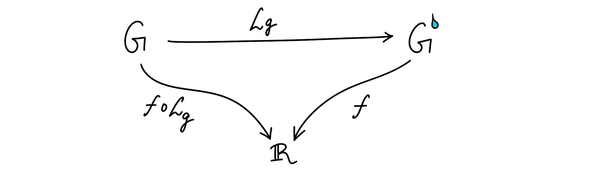
If we view $E_i$ as a vector field on $G$, its pushforward on $G^💧$, $(\mathcal L_{g})_*E_i$, should act on a function $f\in C^\infty (G^💧)$ by mimicking whatever $E_i$ would have done in its place. Given some point $h\in G$, with $\mathcal L_g(h) = gh \in G^💧$, we have

$$\begin{align} \big[(\mathcal L_{g})_*E_i \,f\big](gh) &= \big[E_i(f \circ \mathcal L_g)\big](h) \end{align}$$

Moreover,

$$\begin{align} \big[E_i(f \circ \mathcal L_g)\big](h) &= \frac{d}{dt}[f\circ \mathcal L_g]\big(h \exp(t\tilde E_i)\big)\Big\vert_{t=0}\\ &= \frac{d}{dt}f\big(g h\exp(t\tilde E_i)\big)\Big\vert_{t=0}\\ &= [E_i f](gh)\\ &= [(E_i f)\circ \mathcal L_g](h). \end{align}$$

Now let $G=G^💧$ (as we have done implicitly in the calculation above). Observe that the calculation above involved the following maps:

$$\begin{align} f: G &\rightarrow \mathbb R\\ E_i f : G &\rightarrow \mathbb R\\ \end{align}$$

i.e., $f$ and its derivative. Then, we notice that we can perform either of these maps on $G^💧$ as well. That is, we do $\mathcal L_g: G \rightarrow G$ first, and then perform either of the above maps. This gives us two more maps:

$$\begin{align} f\circ \mathcal L_g: G &\rightarrow \mathbb R\\ (E_i f)\circ \mathcal L_g : G &\rightarrow \mathbb R\\ \end{align}$$

Finally, we note that $E_i$ can act on the function $f\circ \mathcal L_g$, giving us yet another function

$$E_i(f\circ \mathcal L_g): G \rightarrow \mathbb R.$$ That $E_i(f\circ \mathcal L_g)$ and $E_i(f)\circ \mathcal L_g$ are the same function, is what we showed, which is not true unless $E_i$ is left-invariant. The fact that $\mathcal L_g$ moves in and out of the differentiation is what “left-invariant” refers to (also see the commutative square here ). An analogous property is exhibited by $\varepsilon^i$.

🍩 Left-Invariance of Geometric Structure

Now consider what should happen if we define the Riemannian metric of $G$ as

$$\langle \hspace{1pt}\cdot\hspace{2pt},\hspace{1pt}\cdot\hspace{2pt}\rangle = \textrm{k}_{ij}\hspace{1pt}\varepsilon^i \varepsilon^j$$

where $\textrm{k}_{ij}$ are constants that should be thought of as a “weighting matrix”. Clearly, this metric should inherit the left-invariance properties of $(\varepsilon^i)_{i=1}^n$. Indeed, we can use similar arguments as before to show that if $\mathbf v, \mathbf w \in T_gG$, then

$$\langle \mathbf v,\mathbf w\rangle_g = \langle (\mathcal L_h)_{\ast_g}\mathbf v, (\mathcal L_h) _{\ast_g}\mathbf w\rangle _{hg}$$

To see this, we evaluate the right hand side:

$$\begin{align*} \langle (\mathcal L_h)_{\ast_g}\mathbf v, (\mathcal L_h) _{\ast_g}\mathbf w\rangle _{hg} &= \textrm{k}_{ij}\hspace{1pt}\varepsilon^i_{hg} \varepsilon^j_{hg} \big((\mathcal L_h)_{\ast_g}\mathbf v, (\mathcal L_h) _{\ast_g}\mathbf w\big)\\ &= \textrm{k}_{ij}\hspace{1pt}\varepsilon^i_{hg} \big((\mathcal L_h)_{\ast_g}\mathbf v\big) \varepsilon^j_{hg} \big((\mathcal L_h) _{\ast_g}\mathbf w\big)\\ \end{align*}$$

Then, use the duality between pushforwards and pullbacks to show that

$$\begin{align*} \varepsilon^i_{hg} \big((\mathcal L_h)_{\ast_g}\mathbf v\big) &= \big[(\mathcal L_h)^\ast_{_{hg}}\varepsilon^i_{hg}\big] \big(\mathbf v\big) \\ &=\big[(\mathcal L_h)^\ast_{_{hg}} (\mathcal L_{h^{-1}})^\ast_{_g} \varepsilon^i_{g}\big] \big(\mathbf v\big) \\ &= \varepsilon^i_g \big(\mathbf v\big). \end{align*}$$

The notation may seem cumbersome, but given how light-yet-powerful the notation of differential geometry is already, it’s not too bad (depending on what you intend to do with it). Drawing a diagram involving the points $g$ and $hg$, as well as the maps $\mathcal L_g$ and $\mathcal L_h$, can help in understanding the above calculation.

A left-invariant volume form can be defined as $\omega = \varepsilon^1 \wedge \varepsilon^2 \wedge \cdots \wedge \varepsilon^n$, and has analogous invariance properties.

---

🍩 Some Actual Examples

We could also have chosen to work with a coordinate coframe on an open set $U$ containing $g$ in order to express $\langle \cdot, \cdot \rangle$. In this case, we should compute the metric tensor coefficients since they will no longer be trivial. In this post , I computed the metric tensor coefficients for the sphere (not a Lie group!) in spherical polar coordinates. In the next one , I pull back the geometric structure of $SO(3)$ to its axis-angle parametrization .