Integration on SO(3)

I will construct the Haar measure for $SO(3)$ and pull it back to the axis-angle parametrization of orthogonal matrices. The goal is to be able to integrate (and thereby define probability densities) on $SO(3)$. My earlier post on the Riemannian volume form is a prerequisite, though you could also just skip over any equations involving exterior calculus (distinguished by the use of the “$\wedge$” operation) and focus on the computations done in axis-angle coordinates.

The Riemannian Volume Form

Let the basis for $\mathfrak{so}(3)$ be given by

\[ \begin{align*} \tilde E_1 &= \begin{bmatrix*}[r] 0 & 0 & 0 \\ 0 & 0 & -1 \\ 0 & 1 & 0 \end{bmatrix*} \\ \tilde E_2 &= \begin{bmatrix*}[r] 0 & 0 & 1 \\ 0 & 0 & 0 \\ -1 & 0 & 0 \end{bmatrix*} \\ \tilde E_3 &= \begin{bmatrix*}[r] 0 & -1 & 0 \\ 1 & 0 & 0 \\ 0 & 0 & 0 \end{bmatrix*} \end{align*} \]

and the corresponding dual basis of $\mathfrak{so}(3)^*$ be given by $\lbrace \tilde \varepsilon^1, \tilde \varepsilon^2, \tilde \varepsilon^3\rbrace$, where we recall that $\tilde \varepsilon^i$ is like the `row vector’ counterpart to $E_i$. In particular, $\tilde \varepsilon^i(\tilde E_j) = \delta_{ij}$. As usual, we will push these vectors and covectors around using the left-multiplication maps of the group to generate $\lbrace E_i\rbrace_{i=1}^3$ and $\lbrace \varepsilon^i\rbrace_{i=1}^3$. Once again, $\varepsilon^i(E_j) = \delta_{ij}$, but now $\delta_{ij}$ must be thought of as a smooth function on $SO(3)$ that is constant-valued.

The Haar measure on $SO(3)$ is denoted by $\mu$. It is (up to scaling) the canonical¹ Riemannian volume form on $SO(3)$ determined by the left-invariant metric on $SO(3)$:

$$ \mu = \textrm c\cdot \varepsilon^1\wedge\varepsilon^2\wedge\varepsilon^3 $$

where $\textrm c\in \mathbb R_{>0}$ is a normalizing constant (that we will compute later) satisfying

$$ \int_{SO(3)}\mu = 1. $$

This normalization procedure makes sense precisely because $SO(3)$ is a compact manifold. Note that $\mu$ is also a probability measure and defines a ‘uniform distribution’ over the space of rotations.

As an engineer by training, my goal is to do calculations involving $\mu$. Sadly, this often requires us to step away from the intrinsic formulation and work with coordinate charts instead. The good news is that we can come back to the intrinsic formulation when we want to prove theorems and do manipulations that are intrinsic to $SO(3)$. It is important to remember that the coordinate-based approach that will embark on will be oblivious to many of the topological and group-theoretic properties of $SO(3)$. It will of course respect the local Riemannian structure of $SO(3)$… it better!

---

Axis-Angle Parametrization

Recall that any rotation of $\mathbb R^3$ is given by an axis and an angle of rotation. These are represented by tuples of the form $(\mathbf u, \theta)$, where $\mathbf u\in S^2\subseteq \mathbb R^3$ is a unit vector² and $\theta\in [0, \pi]$. This gives the axis-angle parametrization of $SO(3)$:

\[ \begin{align*} S^2\times [0, \pi] &\to SO(3) \\ (\mathbf u, \theta) &\mapsto \exp\big(\theta\cdot \mathbf u^\wedge\big) \end{align*} \]

where $\mathbf u^\wedge$ denotes the skew-symmetric matrix corresponding to $\mathbf u$ (and has nothing to do with the big wedge ‘$\wedge$’ operation from earlier). We have something even better; the Cayley-Hamilton theorem can be used to simplify the infinite series involved in matrix exponentiation, and so the axis-angle parametrization can be written as

$$ (\mathbf u, \theta) \mapsto \mathbf I + \sin\theta\cdot \mathbf u^\wedge + (1-\cos\theta)\cdot (\mathbf u^\wedge)^2 $$

The following trick will greatly simplify our presentation. What prevents us from calling the above as the axis-angle coordinates (as opposed to parametrization) is that it fails bijectivity when $\theta = 0$ and $\theta = \pi$; all $0$-angle rotations are the same regardless of the axis of rotation, and $\pi$-angle rotations about $\mathbf u$ and $-\mathbf u$ are the same rotation. Either case, $\theta = 0$ and $\theta = \pi$, determines a $2$-dimensional submanifold of $S^2\times [0, \pi]$:

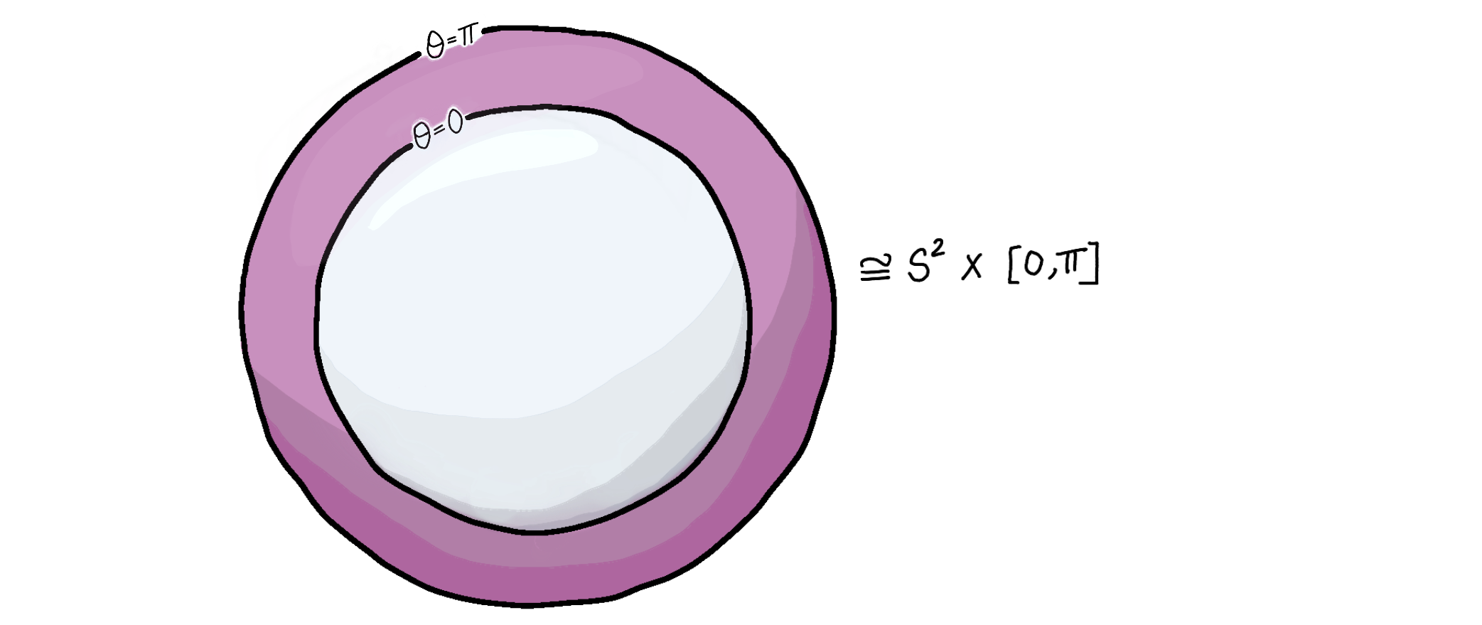
Topologically, the axis-angle parametrization (i) collapses the inner surface of this shell into a single point, and (ii) glues together each pair of antipodal points on the outer surface. So, while the image of the $\theta = 0$ points is a single point in $SO(3)$ (namely, the identity element), the image of the $\theta = \pi$ points is a $2$-dimensional submanifold of $SO(3)$. The aforementioned trick which we will use is that these lower-dimensional sets have measure zero under $\mu$, so we can peel them away from the spherical shell before doing integration and probability. No longer would we have an obstruction to bijectivity.

Let $\widetilde {SO}(3) \subseteq SO(3)$ denote the image of the axis-angle parametrization when restricted to $S^2\times (0, \pi) \subseteq S^2\times [0, \pi]$, so that

$$ \int_{SO(3)} \mu = \int_{\widetilde{SO}(3)}\mu $$

Moreover, we can consider the spherical polar parametrization for $S^2$, which takes values in $[0,2 \pi) \times (0, \pi)$ (after neglecting a similar measure-zero subset!). At long last, we have a bijection on our hands:

\[ \begin{align*} \psi:\quad & U \ \to\ \widetilde {SO}(3) \\ \psi^{-1}:\quad & \widetilde {SO}(3) \ \to\ U\\ \end{align*} \]

where $U = [0, 2\pi)\times(0, \pi)\times (0, \pi) \subseteq \mathbb R^3$. From here on, we will treat the set $U$ as a cube in $\mathbb R^3$ with all but one of its faces removed, i.e., we will quite literally think of it as the set $[0, 2\pi)\times(0, \pi)\times (0, \pi)$ rather than a ‘spherical shell’.

If we blur the technical details that must be checked, then $\psi$ may be called a diffeomorphism, and we can think about pulling back the Riemannian structure of $\widetilde{SO}(3)$ through $\psi$ in order to establish an (almost-global) isometry from $U$ to $SO(3)$³.

Pulling Back the Volume Form

The coordinate chart lets us use integration in $\mathbb R^3$ as a substitute for integration in $SO(3)$:⁴

\[ \begin{align*} \int_{SO(3)} \mu &= \int_{\psi^{-1}\big(\widetilde{SO}(3)\big)} \psi^*\mu\\ &= \int_{U} \psi^*\mu \end{align*} \]

Consider the standard frame of $U\subseteq \mathbb R^3$, $\lbrace \frac{\partial}{\partial x^i}\rbrace_{i=1}^3$, and its dual coframe $\lbrace dx^i\rbrace_{i=1}^3$. Any $3$ form in $U$ (and in particular, $\psi^*\mu$) can be expressed as $f\ dx^1 \wedge dx^2 \wedge dx^3$, where $f\in C^\infty(U)$ is a smooth function. Using Lemma 14.16 of Intro. to Smooth Manifolds,⁵

\[ \psi^*\mu = \textrm c\ (\psi^*\varepsilon ^1)\wedge (\psi^*\varepsilon ^2)\wedge (\psi^*\varepsilon ^3) \]

whereas the pullback $\psi^*\varepsilon ^i$ is given by

\[ \big[\psi^*\varepsilon ^i\big]\Big(\frac{\partial}{\partial x^j} \Big) =\varepsilon ^i\Big(\psi_* \frac{\partial}{\partial x^j} \Big) \]

Actually, we will sneak in the definition of $\varepsilon^i$ here (the motivation for this will be made clear shortly):

\[ \begin{align*} \big[\psi^*\varepsilon ^i\big]\Big(\frac{\partial}{\partial x^j} \Big) =\big[\psi^* (\mathcal L_{g^{-1}})^*\tilde \varepsilon ^i\big]\Big(\frac{\partial}{\partial x^j} \Big) = ?????? \end{align*} \]

So, Proposition 14.9 can be used to yield that

\[ \psi^*\mu = \textrm c\ \textrm{det}(???) \]