Matrix Multiplication

In this post, I want to bridge the gap between abstract vector spaces (which are the mathematical foundation of linear algebra) and matrix multiplication (which is the linear algebra most of us are familiar with). To do this, we will restrict ourselves to a specific example of a vector space – the Euclidean space. Unlike the typical 101 course in linear algebra, I will avoid talking about solving systems of equations in this post. While solving systems of equations served as the historical precedent¹ for mathematicians to begin work on linear algebra, it is today an application, and not the foundation of linear algebra.

For this post, I expect that the reader has come across concepts like linear independence and orthogonal vectors before, and can consult Wikipedia for anything that looks new to them.

The Recipe for $\mathbb R^n$

We write $\mathbb R^n$ as a short-hand for $\mathbb R \times \mathbb R \times \dots \times \mathbb R$, the set of sequences (of length $n$) of real numbers. For notational convenience, we also use ‘$\mathbb R^n$’ to denote the $n$-dimensional Euclidean space, which is not just a set of objects, but a set of objects that has a particular structure. In order to arrive at this structure, we need to introduce the following mathematical ingredients, in order:

1. Scalars: Defined as the elements of a set (technically, a field ) which has two binary operations called addition and multiplication. We choose $\mathbb R$ (the real numbers) as the set of scalars.

2. Vectors: For some integer $n > 0$, we define the set of vectors as $\mathbb R^n$. The vectors have the vector addition and scalar multiplication operations. These operations satisfy certain axioms which ensure that the addition and multiplication operations behave like they ought to.

3. Basis: We need to pick a basis $\mathcal B$ for $\mathbb R^n$, which is a set of vectors $\lbrace \bold b_1, \bold b_2, \dots, \bold b_n \rbrace$, where $\bold b_i \in \mathbb R^n$, such that every vector $\bold v\in \mathbb R^n$ can be uniquely expressed as a linear combination of the basis vectors. This means that there is a unique sequence of real numbers $v^{(\mathcal B)}_1,v^{(\mathcal B)}_2, \dots, v^{(\mathcal B)}_n \in \mathbb R$ satisfying

$$\bold v= v^{(\mathcal B)}_1 \bold b_1 + v^{(\mathcal B)}_2 \bold b_2 + \dots + v^{(\mathcal B)}_n \bold b_n$$

4. Inner Product: For vectors $\bold v$ and $\bold w$, $\langle \bold v,\bold w \rangle$ is called the inner product of $\bold v$ and $\bold w$; it maps each pair of vectors to a scalar. The usual inner product that we define for $\mathbb R^n$ is sometimes called the dot product. An inner product imparts geometry to its vector space, because we can use it to define the ’length’ of a vector $\bold v$ as $\sqrt{\langle \bold v, \bold v\rangle }$, and ‘angles’ between vectors as

$$\theta(\bold v,\bold w) = \arccos\left(\frac{\langle \bold v,\bold w \rangle}{\sqrt{\langle \bold v, \bold v\rangle \langle \bold w, \bold w\rangle}}\right)$$

5. Orthonormal Basis: If the basis $\mathcal B$ is such that $\langle \bold b_i, \bold b_j\rangle = 1$ when $i=j$ and $0$ otherwise, we call it an orthonormal basis. Because of how we defined $\theta$, $\langle \bold b_i, \bold b_j\rangle = 0$ implies that $\theta(\bold b_i, \bold b_j)=90^\circ$.

We have introduced ingredients 3, 4, and 5 in a very specific order. Let’s see why that is so.

---

The Standard Basis

Mathematicians avoid picking the basis $\mathcal B$ explicitly. Often, they start their analysis with the following (implied) disclaimer:

“We have chosen some basis, $\mathcal B \subseteq \mathbb R^n$, but the specific choice of basis does not matter for what we’re about to show.”

Basically, don’t worry too much about which basis we chose, just know that we have chosen one. Once a basis $\mathcal B = \lbrace \bold b_1, \bold b_2, \dots, \bold b_n\rbrace$ has been chosen, each vector $\bold v\in \mathbb R ^n$ can be uniquely expressed by a sequence of $n$ coefficients, $\left(v^{(\mathcal B)}_i\right)_{i=1}^n$, such that $\bold v=\sum_{i=1}^n v^{(\mathcal B)}_i \bold b_i$. Thus, the vector $\bold v$ can be expressed unambiguously using the following, more familiar notation:

$$\begin{bmatrix} v^{(\mathcal B)}_1\\ v^{(\mathcal B)}_2\\ \vdots\\ v^{(\mathcal B)}_n \end{bmatrix}$$

Note that this notation involves both a vector $\bold v$ and a basis $\mathcal B$. Choosing a different basis $\mathcal B’ = \lbrace \bold b’_1, \bold b’_2, \dots, \bold b’_n \rbrace$ changes the coefficients of the vector to $\left(v^{(\mathcal B’)}_i\right)_{i=1}^n$, but it does not change the vector itself. For bases $\mathcal B$ and $\mathcal B’$, we have

$$\bold v=\sum_{i=1}^n v^{(\mathcal B)}_i \bold b_i =\sum_{i=1}^n v^{(\mathcal B')}_i \bold b'_i$$

At a glance, this assertion might appear to contradict with the following observation:

$$\begin{bmatrix} v^{(\mathcal B)}_1\\ v^{(\mathcal B)}_2\\ \vdots\\ v^{(\mathcal B)}_n \end{bmatrix} \neq \begin{bmatrix} v^{(\mathcal B')}_1\\ v^{(\mathcal B')}_2\\ \vdots\\ v^{(\mathcal B')}_n \end{bmatrix}$$

This is purely because of the ‘square-bracket’ notation. Before we write vectors in their ‘square-bracket’ form, we must not only choose a basis, but also fix a basis. Let’s fix a basis $\mathcal B$ for $\mathbb R^n$, which we call as the standard basis. Now, for $c_1,c_2,\dots,c_n\in\mathbb R$, the ‘square-bracket’ notation

$$\begin{bmatrix} c_1\\ c_2\\ \vdots\\ c_n \end{bmatrix}$$

refers unambiguously to the vector $\sum_{i=1}^n c_i \bold b_i$. Therefore, observe that

$$\begin{bmatrix} v^{(\mathcal B)}_1\\ v^{(\mathcal B)}_2\\ \vdots\\ v^{(\mathcal B)}_n \end{bmatrix} \neq \begin{bmatrix} v^{(\mathcal B')}_1\\ v^{(\mathcal B')}_2\\ \vdots\\ v^{(\mathcal B')}_n \end{bmatrix} \text{ \ because\ } \sum_{i=1}^n v^{(\mathcal B)}_i \bold b_i \neq \sum_{i=1}^n v^{(\mathcal B')}_i \bold b_i$$

Thus, there is a distinction between the vector itself and its representation in the standard basis $\mathcal B$; the ‘square-bracket’ notation gives us the latter, and it is our job to infer the former. Observe that the standard basis vectors $\bold b_i$ can themselves be represented in the ‘square-bracket’ notation, as

$$\mathcal B = \left\lbrace \begin{bmatrix} 1\\ 0\\ 0\\ \vdots\\ 0 \end{bmatrix}, \begin{bmatrix} 0\\ 1\\ 0\\ \vdots\\ 0 \end{bmatrix}, \begin{bmatrix} 0\\ 0\\ 1\\ \vdots\\ 0 \end{bmatrix}, \dots, \begin{bmatrix} 0\\ 0\\ 0\\ \vdots\\ 1 \end{bmatrix} \right\rbrace$$

Notice that we can do our usual linear algebra stuff without actually specifying the contents of $\mathcal B$, as long as we fix $\mathcal B$ and don’t change it thereafter. Nothing about the orthogonality of $\bold b_1, \bold b_2, \dots, \bold b_n$ has been said yet, because we need an inner product to even define what orthogonality means.

The Dot Product

We can now define an inner product in terms of the standard basis $\mathcal B$. For vectors $\bold v, \bold w \in \mathbb R^n$, we define $\langle \bold v, \bold w\rangle = \sum_{i=1}^n v^{(\mathcal B)}_i w^{(\mathcal B)}_i$, which we call as the dot product. In the matrix multiplication or “square-bracket” notation, we write this as

$$\begin{bmatrix} v^{(\mathcal B)}_1 & v^{(\mathcal B)}_2 & v^{(\mathcal B)}_3 & \dots & v^{(\mathcal B)}_n \end{bmatrix} \begin{bmatrix} w^{(\mathcal B)}_1 \\ w^{(\mathcal B)}_2 \\ w^{(\mathcal B)}_3 \\ \vdots \\ w^{(\mathcal B)}_n \end{bmatrix}$$

Note that we are defining the inner product this way. Importantly, we are defining it in a way that makes the basis vectors, $\bold b_1, \bold b_2, \dots, \bold b_n$, orthonormal. If we had instead defined the inner product as $\langle \bold v, \bold w\rangle = \sum_{i=1}^n v^{(\mathcal B’)}_i w^{(\mathcal B’)}_i$, then the basis $\mathcal B’$ becomes orthonormal (under this new definition of orthonormality). Thus, any basis can be ‘made orthonormal’ by redefining the inner product appropriately.

The ‘row vector’ corresponding to $\bold v$ is usually called the transpose of $\bold v$, and is denoted as $\bold v^\intercal$. Strictly speaking, it is a linear map $\bold v^\intercal:\mathbb R^n \rightarrow \mathbb R$ (See dual space if you’re curious about what’s going on here.)

---

Linear Algebra

Let $V$ and $W$ be vector spaces. They could be Euclidean spaces, but they could also be subspaces of Euclidean spaces (recall that a flat plane passing through the origin is a subspace of $\mathbb R^3$), or something else entirely. A linear map or a linear transformation is a map $f:V\rightarrow W$ which transforms each vector in $V$ to a vector in $W$ in a linear manner. This means that for $\bold u,\bold v\in V$ and $a\in \mathbb R$,

$$f(\bold u + \bold v)= f(\bold u)+f(\bold v)$$

and

$$f(a\bold u)= af(\bold u)$$

Notably, we have $f(0 \bold u) = f(\bold 0) = \bold 0$. The word ’linear’ comes from the special case of the linear map, $f:\mathbb R \rightarrow \mathbb R$; the plot of this function is a straight line passing through the origin. This is also where the ’linear’ in linear algebra comes from: it is the study of linear maps in vector spaces.

Now here’s where abstract linear algebra starts developing into the ‘matrix multiplication’ version of linear algebra:

Any linear map $f:V \rightarrow W$ between two finite-dimensional vector spaces $V$ and $W$ can be represented as a matrix.

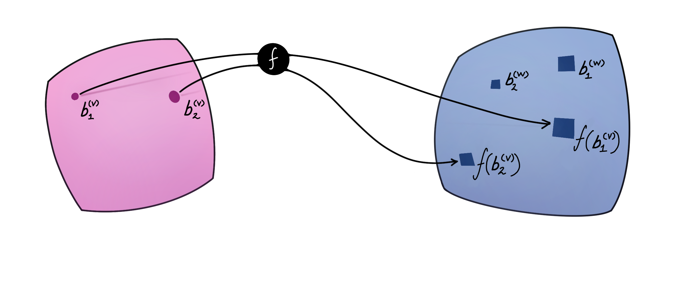
To see this, let’s start by choosing bases for $V$ and $W$, denoted as $\mathcal B^{(V)} = \lbrace \bold b^{(V)}_1, \bold b^{(V)}_2, \dots, \bold b^{(V)}_n \rbrace$ and $\mathcal B^{(W)} = \lbrace \bold b^{(W)}_1, \bold b^{(W)}_2, \dots, \bold b^{(W)}_m \rbrace$, where $n$ and $m$ are the dimensions of $V$ and $W$. For simplicity, we will assume that the scalars in $V$ and $W$ are real numbers (as opposed to, say, one of them being a complex vector space).

Observe that $f(\bold b^{(V)}_i)\in W$. Each vector in the basis of $V$ is mapped (linearly) to a corresponding vector in $W$. This means that we can express each of the mapped basis vectors $f(\bold b^{(V)}_i)$ as a linear combination:

$$\begin{align*} f(\bold b^{(V)}_i) &= F_{1i} \bold b^{(W)}_1 +F_{2i} \bold b^{(W)}_2 + \dots + F_{mi} \bold b^{(W)}_m \\ &= \sum_{j=1}^{m} F_{ji} \bold b^{(W)}_j \end{align*}$$

where $F_{ji} \in \mathbb R$ are unique. Now consider the action of $f$ on an arbitrary vector $\bold v \in V$ that is not a basis vector. We first write $\bold v$ as the linear combination

$$\bold v = v_1 \bold b^{(V)}_1 + v_2 \bold b^{(V)}_2 + \dots + v_n \bold b^{(V)}_n \in V$$

Due to the properties of a linear transformation (i.e., its linearity), we have the following algebra:

$$\begin{align*} f(\bold v) &= f\left(v_1 \bold b^{(V)}_1 + v_2 \bold b^{(V)}_2 + \dots + v_n \bold b^{(V)}_n\right)\\ &= f\big(v_1 \bold b^{(V)}_1\big) + f\big(v_2 \bold b^{(V)}_2\big) + \dots + f\big(v_n \bold b^{(V)}_n\big)\\ &= v_1 f\big(\bold b^{(V)}_1\big) + v_2 f\big( \bold b^{(V)}_2\big) + \dots + v_n f\big(\bold b^{(V)}_n\big)\\ \end{align*}$$

Thus, the action of $f$ on the vector $\bold v$ indirectly depends on the action of $f$ on the basis vectors. We have already seen where $f$ takes the basis vectors of $V$, so let’s plug that in:

$$\begin{align*} f(\bold v) &= \sum_{i=1}^n v_i f(\bold b^{(V)}_i) \\&= \sum_{i=1}^n v_i \sum_{j=1}^{m} F_{ji} \bold b^{(W)}_j \\&= \sum_{j=1}^{m} \sum_{i=1}^n v_i F_{ji} \bold b^{(W)}_j\\ &= \sum_{i=1}^n v_i F_{1i} \bold b^{(W)}_1 + \sum_{i=1}^n v_i F_{2i} \bold b^{(W)}_2 + \dots + \sum_{i=1}^n v_i F_{mi} \bold b^{(W)}_m \end{align*}$$

where $\sum_{i=1}^n v_i F_{1i}$ is the coefficient of $f(\bold v)$ corresponding to the basis vector $\bold b_1^{(W)}$. From here on, it’s only a matter of noticing that we can represent this entire relationship using the “matrix-multiplication” operation:

$$\begin{bmatrix} \sum_{i=1}^n v_i F_{1i}\\ \sum_{i=1}^n v_i F_{2i}\\ \vdots\\ \sum_{i=1}^n v_i F_{mi} \end{bmatrix} = \begin{bmatrix} F_{11} & F_{12} & & \\ F_{21} & F_{22} & & \\ & & \ddots & &\\ & & & F_{mn} \end{bmatrix} \begin{bmatrix} v_1\\v_2\\ \vdots \\ v_n \end{bmatrix}$$

which we can write as “$\bold w = \bold F \bold v$”. There is a subtlety here: on the left-hand side of this equation, we assume the ‘standard basis’ to be $\mathcal B^{(W)}$, whereas for the vector on the right we were using the standard basis $\mathcal B^{(V)}$. Thus, we need to fix both bases (one for $V$ and one for $W$) before the linear transformation can be written, unambiguously, as a matrix multiplication. If the dimensions of $V$ and $W$ are the same, we may pick the same basis on either side.

Observe that we never used the inner product while talking about linear transformations, and thus, we do not claim whether the bases we used above are orthonormal. They are simply linearly independent, as all bases are. In case the basis $\mathcal B^{(V)}$ is orthonormal, then this just means that we can find the coefficients $v_1, \dots, v_n$ very easily: $v_i = \langle \bold v, \bold b_i \rangle$.

Orthonormal Transformations

Let’s now study $\mathbb R^n$ as an inner product space, which is the vector space $\mathbb R^n$ combined with the usual inner product – the dot product.

We say that a matrix $\bold U$ is orthonormal if $\bold U^\intercal \bold U = \bold U \bold U^\intercal = \bold I$. This is closely related to how we say that a set of basis vectors is orthonormal: Suppose $\mathcal B$ is an orthonormal basis, then so is the basis $\mathcal B_U = \lbrace \bold U \bold b_1, \bold U \bold b_2, \dots, \bold U \bold b_n \rbrace$, because

$$\langle \bold U\bold b_i, \bold U\bold b_j \rangle = \bold b_i^\intercal \bold U^\intercal \bold U \bold b_j = \bold b_i ^\intercal \bold b_j = \langle \bold b_i, \bold b_j \rangle$$

Let the underlying linear transformation corresponding to $\bold U$ be denoted as $g:V\rightarrow V$, with $\mathcal B$ being an orthonormal basis for $V$. $\bold U$ is the representation of $g$ in the matrix multiplication form, with respect to the basis $\mathcal B$. Recall the algebra we did earlier:

$$g(\bold v) = g\Big( \sum_{i=1}^n v_i\bold b_i\Big) = \sum_{i=1}^n v_i g(\bold b_i)$$

where we know that the set $\lbrace g(\bold b_1), g(\bold b_2), \dots g(\bold b_n)\rbrace = \mathcal B_U$ is orthonormal. Thus, $\bold v$ and $g(\bold v)$ have the same representation (given by the numbers $v_1, v_2, \dots v_n$) under $\mathcal B$ and $\mathcal B_U$. This is why we can call $\bold U$ a “change of basis” – it keeps the vector’s representation the same, but changes the (orthonormal) basis that we are representing it in. Even if the vector’s representation is same in either basis, the vector itself is changing under $\bold U$:

$$\bold v = \sum_{i=1}^{n} v_i \bold b_i \neq \sum_{i=1}^{n} v_i g(\bold b_i) = g(\bold v)$$

Alternatively, we can re-express the transformed vector in the original basis $\mathcal B$, in which case $g$ is interpreted as purely a transformation of the vector’s components while keeping the basis fixed. This duality in how we can view a ‘change of basis’ has been explored more in this article .

Preserving Structure and Dimension

Any transformation on a mathematical space that preserves its structure (i.e., the relationships of its objects to each other) turns out to be quite special. Linear transformations preserve the structure of a vector space, because any three vectors $\bold u,\bold v,\bold w\in V$ which have the relationship $\bold u + \bold v = \bold w$ are still related to each other after the transformation: $f(\bold u) + f(\bold v) = f(\bold w)$.³

Structure-preserving transformations which are also invertible are called as isomorphisms . We can show that the inverse $f^{-1}:W\rightarrow V$, if it exists, must also be a linear transformation. Thus, $f^{-1}$ can be represented as a matrix. Invertible linear transformations are the isomorphisms of vector spaces. Invertible matrices are “square” because a linear transformation can only be invertible if its domain and codomain have the same dimension. ⁴

Similarly, orthonormal matrices represent the structure-preserving transformations in inner-product spaces : a set of vectors that is orthonormal before the transformation remains orthonormal after the transformation, where orthonormality is defined via the dot product. They are also the isomorphisms of inner-product spaces, because the inverse of an orthonormal matrix $\bold U$ always exists $–$ it is $\bold U^\intercal$.

Mathematicians almost always (or perhaps, always) study mathematical objects “up to isomorphism”. This means that we are not studying any particular mathematical object, but rather we are simultaneously studying all of the mathematical objects that are isomorphic to each other. This is why we do not need to specify which basis we are using as the standard basis: it simply does not matter, as long as we fix this basis and stay consistent. This is analogous to how we may need to fix the origin when studying ‘displacement’ and ‘speed’ in physics. Choosing a different origin does not change the physical phenomenon, it only changes our description of it.