Over the past year, I have struggled to pin down what the scope of my blog should be. There is plenty of exposition out there on just about every aspect of modern mathematics, but especially on exterior calculus and differential geometry due to their situation at the intersection of several areas in theoretical and applied mathematics. (As a case in point, the two main references that I’ve been using to self-learn differential forms were the creations of a theoretical physicist and a computer scientist , respectively). So then what is the scope of my blog? Maybe it is for me to catalog the process of self-learning mathematics as an engineering major who lacks a curricular background in modern mathematics. Maybe it is to assure others like me (who are also privileged enough to learn mathematics in isolation of such material concerns as its ‘job prospects’) that it can be done. This post will do a bit of both; it serves in part the purpose of organizing my own thoughts on these matters, and in part the purpose of providing a roadmap for others who are interested in embarking on a similar journey.

To appreciate the aspects of vector fields that I will touch upon requires at least a familiarity with the abstract/modern definition of a vector space. Moreover, one should at least be so far in their mathematics education so as to find the word abstract joyous and exciting as opposed to daunting. An even more pressing prerequisite is perhaps the notion of a smooth (i.e., differentiable) manifold, as it provides if nothing else a concrete mental image to work with. Unless you are already familiar with manifolds, or choose to push forth so daringly with the intention of learning about manifolds later on, I delegate your introduction of manifolds to The Bright Side of Mathematics , one of the best math channels on YouTube. Aspects of topology and differentiability will not show up until the latter half of this discussion.

---

Preliminaries

The Coordinate-Free Approach

The undergrad course on linear algebra at IIT Madras (my alma mater) relies heavily on coordinates. Or maybe it did not emphasize enough the distinction between vectors and their representations via coordinates , so that I was not privy to the underlying structure of vector spaces until very recently. My fond dislike for coordinate-based linear algebra probably stems from this, though I think there’s a case to be made for (to quote one of my mathematical progenitors) speaking as many different languages as one can. This allows one to see the same mathematical object from different perspectives, not unlike how one walks around a sculpture at an art exhibit, appreciating not only the finer details of the craftsmanship but also the overall intent.

The coordinate-based approach to linear algebra begins by choosing (often implicitly) a basis called the standard basis for each vector space that is encountered. It is once we have fixed the choice of the standard basis that we forget (typically for notational convenience) that a basis was ever in need of being chosen. We instead resort to dealing solely with the coordinate representations of the vectors. This is not a bad thing by any means, it provides a two-pronged (algebraic $+$ numerical) framework for analyzing linear transformations by way of matrix multiplication, something that underlies a lot of the modern-day engineering marvels. The case for the coordinate-free approach is then that it reveals the underlying structure of the vector space by breaking free of the shackles of a fixed basis. Indeed, some of the most influential ideas in classical and quantum physics were arrived at by recognizing that no frame of reference is more canonical than the other. The fact that the laws of physics don’t change when we switch from one frame of reference to another leads to the famous conservation laws of physics; see Noether’s theorem. By requiring that the speed of light remain unchanged while switching frames of reference, Einstein was able to uncover key insights that contributed to his theory of special relativity.¹ In a similar vein, by requiring that a vector remain unchanged under a change of basis, we arrive at a rich algebraic and geometric structure that is ripe for mathematical exploration.

Covariance and Contravariance

As Einstein did with the speed of light in his development of special relativity, let us recognize that a vector (not to be confused by the coordinate representation of a vector) will remain unchanged under a change of basis. Letting $\mathbf v = v^1\mathbf e_1 + v^2\mathbf e_2 + \dots + v^n\mathbf e_n$ be a vector in an $n$-dimensional real vector space $V$, where $\mathbf e_1$ through $\mathbf e_n$ are a basis for $V$, we can introduce the following notation:

\[ \begin{align} \mathbf v = \begin{bmatrix} v^1 & v^2 & \dots & v^n\end{bmatrix} \begin{bmatrix} \mathbf e_1 \\ \mathbf e_2 \\ \vdots \\ \mathbf e_n \end{bmatrix} \end{align} \]

Given an invertible matrix $\mathbf A$, we see that

\[ \begin{align} \mathbf v &= \begin{bmatrix} v^1 & v^2 & \dots & v^n\end{bmatrix} \mathbf A^{-1} \mathbf A \begin{bmatrix} \mathbf e_1 \\ \mathbf e_2 \\ \vdots \\ \mathbf e_n \end{bmatrix}\\ &= \left(\mathbf A^{-1}\begin{bmatrix} v^1 \\ v^2 \\ \vdots \\ v^n\end{bmatrix}\right)^\top \mathbf A \begin{bmatrix} \mathbf e_1 \\ \mathbf e_2 \\ \vdots \\ \mathbf e_n \end{bmatrix} \end{align} \]

This hints at a recurring idea in vector and tensor algebra, that the components (or coordinates) of a vector transform in an opposite way to that of the basis vectors. In the language of tensor algebra, we say that the basis vectors transform in a covariant manner, whereas its components transform in a contravariant manner. Here, co- and contra- are supposed to work as antonyms, although beware that the prefix co- is used rather inconsistently² in the larger context of mathematics and English. As the basis vectors and the components of $\mathbf v$ both transform in opposite ways, the vector $\mathbf v$ remains unchanged.³

This is analogous to what would happen if you were measuring the length of a rubber band with a ruler made of rubber. Suppose you measured its length as $1\textrm{cm}$ on Tuesday and $2\textrm{cm}$ on Thursday, what can be deduced about the state of affairs on Thursday? Well, maybe somebody stretched the rubber band to twice its size and held it there, causing the length measurement to increase. Alternatively, they might have painstakingly compressed the ruler to half its length, achieving the same increase in the length measurement. These opposing viewpoints of the same phenomenon are ones that we should become comfortable walking back and forth between. It is a manifestation of the idea of duality that shows up quite often in mathematics. While the notion of duality is fundamental enough that it persists even across a coordinate-heavy treatment of vector spaces, it is brought to the forefront in the modern approach to linear algebra.

Duality

As soon as we define a vector space $V$, we receive ‘for free’ another vector space that is associated with it, denoted as $V^*$, which is called the dual space of $V$. Each element of $V^*$ is a linear function that maps the vectors of $V$ to its underlying field, which in our case is the real numbers. Thus, if $w:V \rightarrow \mathbb R$ and $w\in V^*$, this means that (by the linearity of $w$)

\[ \begin{align} w(\mathbf v + \mathbf w) &= w(\mathbf v) + w(\mathbf w) \\ w(t \mathbf v) &= t w(\mathbf v) \end{align} \]

where $t\in \mathbb R$ and $\mathbf v, \mathbf w \in V$. Given $v, w \in V^*$, their addition is defined by the rule $(v+w)(\cdot) = v(\cdot) + w(\cdot)$, and scalar multiplication is defined similarly. Thus, $V^*$ is indeed a vector space. The object $w\in V^*$ is called a dual vector, a covector, a linear functional, a linear form, or a one-form . In contrast, the object $\mathbf v \in V$ is called a vector or a one-vector.

Suppose that the vector space $V$ is endowed with an inner product, $\langle \cdot, \cdot \rangle:V\times V \rightarrow \mathbb R$. The inner product is by definition (and therefore, by construction) linear in each of its arguments. So, given a vector $\mathbf v\in V$, the mapping $\langle \mathbf v, \cdot \rangle:V \rightarrow \mathbb R$ passes all the requirements for its membership in $V^*$. Let’s define $\mathbf v^\flat (\cdot)=\langle \mathbf v, \cdot \rangle$ such that $\mathbf v^\flat\in V^*$. The inner product thus induces a mapping $\mathbf v \mapsto \mathbf v^\flat$ that associates each vector $\mathbf v$ with a corresponding covector $\mathbf v^\flat\in V^*$. Conversely, we can associate to each covector $f$ a vector $f^\sharp \in V$, which is the vector that satisfies $\langle f^\sharp, \mathbf v\rangle = f(\mathbf v)$.

We say that $V$ and $V^*$ are isomorphic (i.e., have the same underlying structure) as vector spaces, and use ‘$\sharp$’ and ‘$\flat$’ (which are called the musical isomorphisms ) to ’translate between the languages’ of the two vector spaces. In high school and undergraduate linear algebra, we might have written $\mathbf v^\top$ to refer to the dual version of (i.e., the covector that is paired to) $\mathbf v$ (it helps that ‘covector’ rhymes with ‘row-vector’). The musical isomorphisms generalize the notion of a transpose by permitting it to operate differently in either direction. The musical meaning of ‘$\sharp$’ and ‘$\flat$’ (raising/lowering a note) is still relevant; it corresponds to the raising/lowering of indices. Take a look again at $(1)$, and see that I have used the choice of index (superscript vs. subscript) to distinguish the contravariant and covariant pieces.

Topology

All of the above was introduced in the absence of a smooth manifold, which suggests that manifolds are yet to contribute something to the discussion. Before we proceed, I’d like to list some concepts that I think you should at least skim the Wikipedia pages of (and/or YouTube videos on ) before proceeding further:

1. A topological space as a set combined with a collection of open sets
2. The so-called standard topology on $\mathbb R^n$, defined in terms of open balls/neighborhoods
3. Charts and smooth structures on topological spaces; a cursory understanding of the jargon should be sufficient for our purpose (which is to have fun)
4. Homeomorphisms (and diffeomorphisms), which are continuous (differentiable) maps that have continuous (differentiable) inverses

These topics are also covered in the first chapter of Introduction to Smooth Manifolds , by John M. Lee.

An often overlooked requirement for studying differential geometry is the ability to conceptualize the composition of functions. Given $f_1:A \rightarrow B$ and $f_2:B \rightarrow C$, their composition $f_2 \circ f_1:A \rightarrow C$ can be read out aloud as ‘$f_2$ after $f_1$’. It is the composition of $f_1$ with $f_2$. The order in which $f_1$ and $f_2$ appear in the preceding statements is a source of confusion that can be eliminated by drawing some arrow diagrams. Alternatively, remember that $f_2 \circ f_1 (\cdot) = f_2\left(f_1(\cdot)\right)$, so the functions must be ordered such that the image of $f_1$ is contained in the domain of $f_2$. Finally, $C^1(\mathcal D)$ is the set of all functions that are defined on the domain $\mathcal D$ whose first derivative is continuous (i.e., are differentiable). A function is said to be smooth if it’s in $C^\infty (\mathcal D)$, though the distinction between $C^1$ and $C^\infty$ is not entirely relevant given the rigor of this article.

---

Tangent & Cotangent Spaces of $\mathcal M$

Any $n$-dimensional vector space is isomorphic to $\mathbb R^n$, which is to say that it can only differ superficially from $\mathbb R^n$. This begs the question of what happens in $n$-dimensional spaces that differ from $\mathbb R^n$ in some meaningful way. Of particular interest to us (and to physicists and roboticists) are spaces that are curved. Einstein was interested in the geometry of a particular curved four-dimensional space (composed of one temporal and three spatial dimensions). A prototypical example to keep in mind is the surface of a ball in $\mathbb R^3$, which is a $2$-dimensional manifold; each point on its surface has a neighborhood that appears to be a $2$-dimensional plane (hence arises the confusion of flat-earthers).

The Tangent Space at $p$

An $n$-dimensional manifold has the property that it locally (but not necessarily globally) resembles (i.e., is homeomorphic to) the $n$-dimensional Euclidean space. We will denote throughout an arbitrary manifold by $\mathcal M$. At each point $p\in \mathcal M$, there is (at least one) chart $(U, h)$ such that $U\subseteq \mathcal M$ is an open set containing $p$ and $h:U\rightarrow U^\prime$ maps the points in $U$ to those in an open set $U^\prime \subseteq \mathbb R^n$. We say that the manifold is differentiable if the given collection of charts constitutes a smooth atlas; a smooth atlas is a collection of charts that are compatible with each other in a way that lets us (unambiguously) walk back and forth between $\mathcal M$ and its local descriptions in $\mathbb R^n$ for all our differentiation purposes.

The points on $\mathcal M$ do not constitute a vector space, as we don’t necessarily know what it means to ‘add two points on a manifold’, and vector spaces must (amongst other things) have addition. Given a chart $(U, h)$, $h(U)\subseteq U^\prime$ is not a vector space either (as it’s not necessarily closed under addition). It will take some more effort to define a vector space at each point $p$ of $\mathcal M$, which will be called the tangent space of $\mathcal M$ at $p$, and denoted $T_p \mathcal M$. A naive (and potentially misleading) picture of the tangent space is that of a hyperplane touching $\mathcal M$ at $p$. A more rigorous picture is given by the following diagram:

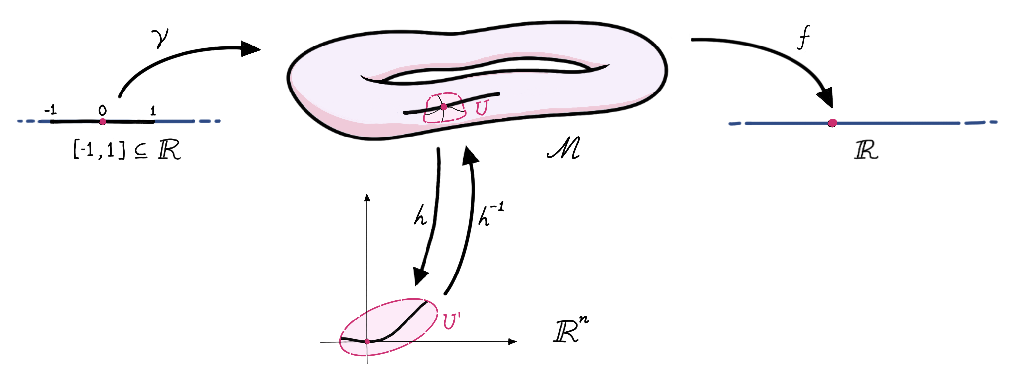
Here, $\gamma:[-1,1] \rightarrow \mathcal M$ is a differentiable map (in the sense that $h\circ \gamma:[-1,1]\rightarrow \mathbb R^n$ is differentiable). As we vary $t\in[-1,1]$, $\gamma(t)$ traces out a path (or a curve⁴) on $\mathcal M$. $f:\mathcal M \rightarrow \mathbb R$ is an arbitrary differentiable function on $\mathcal M$ (written as $f \in C^1(\mathcal M)$) whose arbitrariness will play a key role in our construction of tangent vectors.

Let $\gamma(0)=p$ and $\gamma(\epsilon)=p^\prime$ for some $0<\epsilon \approx 0$. The idea of ‘differentiation on manifolds’ is to capture the change in the value of $f$ as we move from $p$ to $p^\prime$. The choice of the map $\gamma$ (subject to the constraint that it is differentiable and that $\gamma(0)=p$) decides how fast, and in what direction $\gamma(t)$ crosses $p$, leading to the notion of a directional derivative at $p$. A path $\tilde \gamma$ might zip past $p$ twice as fast as $\gamma$, such that $\tilde \gamma(\epsilon/2) = p^\prime$, i.e., $\tilde \gamma$ took only ‘half as much time’ as $\gamma$ to get from $p$ to $p^\prime$. One way to do this is to define $\tilde \gamma(t)=\gamma(2t)$, which speeds up the evolution of time by a factor of $2$. Thus, by allowing time to elapse faster, slower, or backward, we have something resembling the scalar multiplication of vectors.

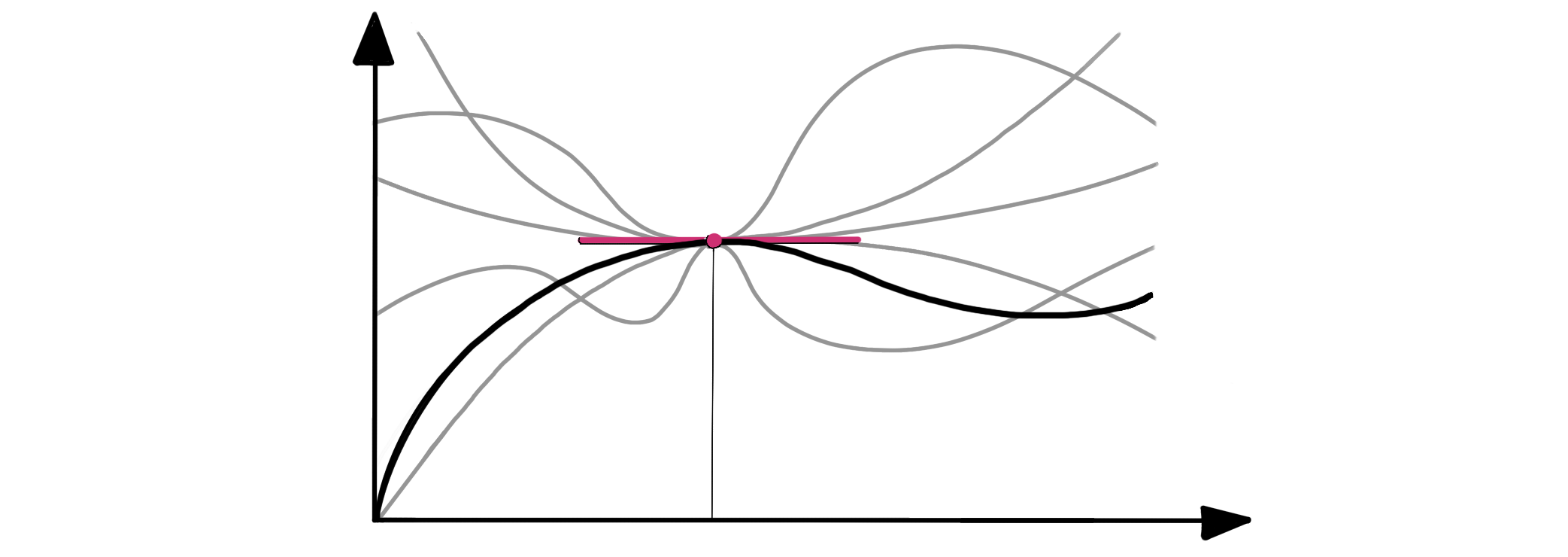
However, the paths (or functions) $\gamma$ themselves are not the tangent vectors. This is because the tangent space at $p$ is not concerned with how the paths behave away from $p$, rather, it looks at how the infinitesimal displacements near $p$ change the value of an arbitrary smooth function $f$. A suitable definition of a tangent vector is as the equivalence class of (i.e., the set of all) paths that zip past $p$ with the same direction and speed; each of these paths corresponds to the same tangent vector as the paths are indistinguishable near $p$. Similarly, our usual notion of a tangent of a function has an alternative interpretation: it is identified with the set of all functions whose first-order Taylor series approximations agree (at a given point):

Given a tangent vector $\mathbf v\in T_p \mathcal M$, we can pick a representative path $\gamma$ from its equivalence class to give a tangible meaning to $\mathbf v$. In particular, given any real-valued smooth function $f\in C^1(\mathcal M)$, the directional derivative corresponding to $\mathbf v$ is denoted by

\[ \begin{align} \mathbf v(f) = \frac{d}{dt}[f\circ\gamma (t)]_{t=0} \end{align} \]

By construction, $\mathbf v(f)$ does not depend on the particular choice of $\gamma$ from the equivalence class of $\mathbf v$. Observe also, that $\mathbf v(f)\in \mathbb R$, which suggests that the function $f$ plays a role similar to that of a covector/dual vector.

The Cotangent Space at $p$

The fact that $\mathbf v(f)\in \mathbb R$ is to be compared to our earlier observations about covectors. A covector is an object that reduces vectors to real numbers. More formally, it is a linear function whose domain is the entire vector space (in this case, $T_p\mathcal M$) and whose codomain is the underlying field of scalars (in this case, $\mathbb R$). So is a function $f\in C^1(\mathcal M)$ a covector? Not quite.

We could not simply identify the tangent vectors with the paths/curves on $\mathcal M$ passing through $p$ because it would lead to inadvertent double-counting; two paths that are indistinguishable near $p$ would get counted as two distinct tangent vectors, which is not the case. A similar problem arises if we try to identify the functions $f\in C^1(\mathcal M)$ with covectors. Two functions that behave similarly near $p$ would get counted as different cotangent vectors, even though they extract the same measurement out of a given vector.

So, we do the same thing as before. Denote by $df$ a cotangent vector, covector, or one-form at $p$, defined as the equivalence class of all the functions that have the same directional derivatives at $p$. In other words, functions $f_1,f_2\in C^1(\mathcal M)$ are associated to the same covector $df$ as long as $\mathbf v(f_1) = \mathbf v(f_2)$ for all $\mathbf v \in T_p \mathcal M$. Since $df$ is itself something that operates on vectors, we define $df$ such that its operation on the vectors is given by $df(\mathbf v) = \mathbf v(f)$, where the $f$ can be any representative from the equivalence class of $df$. The set of all covectors at $p$ make up the cotangent space of $\mathcal M$ at $p$, which is denoted as $T^*_p\mathcal M$ on account of its duality to $T_p\mathcal M$.

For example, if $\mathcal M=\mathbb R$, then $T_p \mathbb R$ is a one-dimensional vector space that encapsulates how fast we are moving past $p\in \mathbb R$, and whether our movement is to the left or to the right; the directions left and right are related by a change of sign. In this case, $T^*_p \mathbb R$ can be identified with the set of all slopes that a Taylor series approximation of some function (at $p\in\mathbb R$) could have. Its dimension is also one, as the only choice of freedom here is the slope of the line. Before moving on from this example, reflect upon what a path $\gamma :[-1,1]\rightarrow \mathbb R$ on this manifold might possibly look like.

Partial Derivatives and Differentials

In the diagram above (which must be consulted repeatedly during the forthcoming discussion), we depict the standard basis on $\mathbb R^n$ by the black rays. Since $h$ is a homeomorphism, we can use $h^{-1}$ to lift the black rays onto $\mathcal M$. These gives us ‘coordinate paths’ on $\mathcal M$ whose equivalence classes (at each $p\in U$) may be defined as a basis of $T_p \mathcal M$ (for each $p\in U$). The basis thus obtained at $p$ is commonly denoted as $\big(\frac{\partial}{\partial x^i}\big\rvert_p\big)_{i=1}^n$, whereas $\big(\frac{\partial}{\partial x^i}\big)_{i=1}^n$ defines a set of $n$ vector fields on $U$, called as a local coordinate frame. The discussion of frames is deferred to a later post .

An arbitrary vector $\mathbf v \in T_p \mathcal M$ can therefore be expressed as

\[ \begin{align} \mathbf v= v^1 \frac{\partial}{\partial x^1}\Big\rvert_p + v^2 \frac{\partial}{\partial x^2}\Big\rvert_p + \dots + v^n \frac{\partial}{\partial x^n}\Big\rvert_p, \end{align} \]

with $v^i\in \mathbb R$.

The basis $\left\lbrace \frac{\partial}{\partial x^1}\big\rvert_p, \dots, \frac{\partial}{\partial x^n }\big\rvert_p\right\rbrace$ of $T_p \mathcal M$ gives rise to a corresponding basis of $T^*_p \mathcal M$, called the dual basis. The dual basis is denoted as $\left\lbrace dx^1_p, \dots, dx^n_p\right\rbrace$ and defined such that the following identity holds:

\[ \begin{align} dx^i_p\left(\frac{\partial}{\partial x^j}\Big\rvert_p\right) = \delta_{ij}, \end{align} \]

where $\delta_{ij}$ is the Kroenecker delta . A covector $df_p \in T^*_p \mathcal M$ can therefore represented as

\[ \begin{align} df_p = f_1 dx^1_p + f_2 dx^2_p + \dots + f_n dx^n_p. \end{align} \]

The notation that was introduced above starts to have further meaning once we introduce the so-called coordinate functions. Decompose the chart $h$ into its constituent coordinate functions as follows:

\[ \begin{align} h(\cdot)=\begin{bmatrix} x^1(\cdot)\\ x^2(\cdot)\\ \vdots \\ x^n(\cdot) \end{bmatrix} \end{align} \]

such that $x^1(p^\prime), \dots, x^n(p^\prime)$ are the coordinates of a point $p^\prime \in U$ with respect to the chart $(U, h)$ at $p$. Thus, $x^i:U \rightarrow \mathbb R$. It appears as if we have defined the basis vector $dx^i_p$ such that

\[ \begin{align} dx^i_p\Big(\frac{\partial}{\partial x^j}\Big\rvert_p\Big) = \frac{\partial}{\partial x^j}\Big\rvert_p(x^i), \end{align} \]

which is indeed the case, i.e., $x^i$ is a representative function from the equivalence class of $dx^i_p$ (in fact, this statement holds for all $p\in U$).

The Euclidean Case

When $\mathcal M = \mathbb R^n$, there is a canonical inner product on $T_p\mathbb R^n$ that has a diagonal/Dirac delta structure,

\[ \begin{align} \langle \frac{\partial}{\partial x^i}\Big\rvert_p, \frac{\partial}{\partial x^j}\Big\rvert_p\rangle = \delta_{ij}, \end{align} \]

called the Euclidean or flat inner product. Since $dx^i_p\big(\frac{\partial}{\partial x^j}\Big\rvert_p\big) = \delta_{ij}$ also, we have (in the Euclidean case),

\[dx^i_p = \frac{\partial}{\partial x^i}\Big\vert_p^{\flat}, \quad {dx^i_p}^\sharp = \frac{\partial}{\partial x^i}\Big\vert_p. \]

We also have the following convenient fact that follows from the bilinearity of the inner product:

\[ \begin{align} \langle \frac{\partial}{\partial x^i}\Big\rvert_p, \mathbf v\rangle = \sum_{j=1}^{n}v^j \langle \frac{\partial}{\partial x^i}\Big\rvert_p, \frac{\partial}{\partial x^j}\Big\rvert_p\rangle = v^i \end{align} \]

This is analogous to how a row vector such as $\begin{bmatrix}0 & \cdots& 0 & 1 & 0 & \cdots \end{bmatrix}$ picks out the corresponding component of a vector that it operates on. Similarly (by the linearity of ‘$\sharp$’),

\[ \begin{align} \langle \frac{\partial}{\partial x^i}\Big\rvert_p, df^\sharp_p\rangle = f_i. \end{align} \]

Using simple manipulations, we can offer alternative interpretations to the previous equation:

\[ \begin{align} \langle \frac{\partial}{\partial x^i}\Big\rvert_p, df^\sharp_p\rangle &= \langle df^\sharp_p, \frac{\partial}{\partial x^i}\Big\rvert_p\rangle \\ &= ({df_p^\sharp})^\flat \left(\frac{\partial}{\partial x^i}\Big\rvert_p\right)\\ &= {df}_p \left(\frac{\partial}{\partial x^i}\Big\rvert_p\right)\\ &= \frac{\partial}{\partial x^i}\Big\rvert_p(f) = f_i. \end{align} \]

Now behold, for something striking will occur when we combine (8) and (18):

\[ \begin{align} df_p &= \sum_{i=1}^n f_i dx^i_p \\ &= \sum_{i=1}^n \frac{\partial f}{\partial x^i}\Big\rvert_p dx^i_p \end{align} \]

This is nothing but the multivariable chain rule, which relates the differential of a function to infinitesimal changes in its arguments.

It should be noted that the measurement of a vector by a covector can be defined in the absence of an inner product, but we do need an inner product to be able to make sense of the musical isomorphisms.

The Non-Euclidean Case

While it’s always possible to choose a chart $(U, h)$ containing $p$ such that $\frac{\partial}{\partial x^i}\big\rvert_p$ is orthonormal, it is seldom possible to choose an ‘orthonormal coordinate system’ whose coordinate vector fields are orthonormal at all points of $U$. Alternatively, the existence of such a chart would imply that the manifold is of a very special type: it is flat. Cylinders, cones, and other objects that can be wrapped with a sheet of paper without tearing, wrinkling, or folding the paper are examples of flat manifolds. I touch upon this point in a later post . Such considerations will only arise when we try to extend the basis of $T_p \mathcal M$ into a frame, so the reader need not dwell on this point too much right now.

A Riemannian metric $g_{(\cdot)}$ is an object that takes as input a point $p\in \mathcal M$ to become an inner product on $T_p \mathcal M$, written as $g_{p}(\cdot, \cdot)$ or $\langle \cdot,\cdot\rangle_p$ depending on the author. What we have done above is to stipulate that $g_{p}(\frac{\partial}{\partial x^i}, \frac{\partial}{\partial x^j})=\delta_{ij}$. More generally, one introduces a convenient coordinate system on $U\subseteq \mathcal M$ (for instance, the spherical polar coordinates of a sphere ) and then specifies (or when there is some natural choice of metric, computes) the ‘components of the metric tensor’, collected into a matrix of numbers, $g_{ij}(p)$. Each of these components is required to be a smooth function of $p$ – a requirement that marries the differential structure of $\mathcal M$ to its geometric structure. In the general case, we write

\[ \big\langle\frac{\partial}{\partial x^i}, \frac{\partial}{\partial x^j}\big\rangle _p=g_{ij}(p) \]

When stored as the entries of a matrix, $g_{ij}(p)$ are related to the Jacobian matrix of the parameterization evaluated at $p$, and the corresponding determinant tells us how much the parameterization stretches or squishes the space near $p$. There are other ways to compute $g_{ij}(p)$; for instance, when the manifold is not parameterized but given by an implicit equation (such as ‘$x^2 + y^2 + z^2=0$’), it is not clear which Jacobian must be evaluated. See the books by G. S. Chirikjian for more details about these computations.

Tangent/Cotangent Bundles

A fiber bundle is obtained when at each point on a space, a fiber is attached. This is sort of like how hair grows all over your (or at least my South Indian) skin, in which case one of the strands of hair (serving as a representative example of the other strands) gets called the fiber, and the surface of the skin is called the base space. More rigorously, we refer to the following picture from Wikipedia of a fiber bundle:

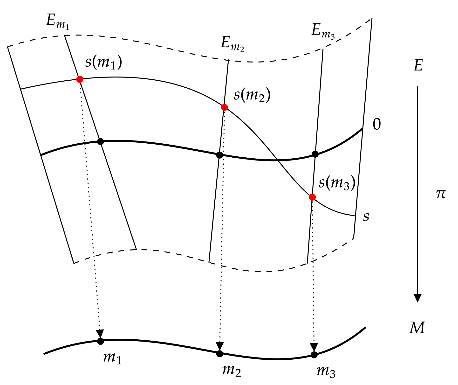
Here, the base space $M$ is a set of points. The squiggly rectangle $E$ is called the total space, and the fiber is a vertical line (not shown). By affixing a copy of the fiber (the vertical line) at each point on $M$ ($E_{m_1}$ on $m_1$, $E_{m_2}$ on $m_2$, and so on) in a particular way, we obtain the total space $E$. Here, $\pi:E\rightarrow M$ is called the projection, which takes a point on the total space to the point on the base space to which a fiber was attached; $s:M\rightarrow E$ is called a section (or more intuitively, a cross-section). The section is a smooth function that chooses at each point of $M$ (e.g., $m_1, m_2, \dots$) a single point on its fiber (e.g., $s(m_1) \in E_{m_1}$, $s(m_2)\in E_{m_2}$, and so on).

A similar characterization allows us to introduce the notion of the tangent bundle of $\mathcal M$, denoted as $T\mathcal M$. The base space is $\mathcal M$, and the object attached at point $p\in \mathcal M$ is the tangent space $T_p \mathcal M$. The projection $\pi:T\mathcal M \rightarrow \mathcal M$ is defined as $\pi(\mathbf v) = p$ where $\mathbf v \in T_p \mathcal M$. Similarly, we can define the cotangent bundle of $\mathcal M$, and denote it as $T^*\mathcal M$.

A section of $T\mathcal M$ is a map that assigns to each point $p\in \mathcal M$ a tangent vector $\mathbf v \in T_p \mathcal M$ (refer to the diagram above). A (smooth) section of the tangent bundle is called a (smooth) vector field. A (smooth) section of the cotangent bundle is called a differential one-form. A more intuitive name for a differential one-form is a ‘smooth one-form field’, but the less intuitive name prevails in the literature, so we might as well acquaint ourselves with it.

Now to unpack the newly introduced objects. A smooth vector field is a function $X:\mathcal M \rightarrow T\mathcal M$ such that $X(p)\in T_p\mathcal M$. One can imagine $X$ as representing the motion of water on $\mathcal M$. After dropping a paper boat at some point on $\mathcal M$, we may sit back and observe where the motion of the water takes it. Once the boat traces out a path on $\mathcal M$, the resulting path is called an integral curve or (rather suitably) a flow on $\mathcal M$ generated by $X$.⁵ The set of smooth vector fields is itself a vector space, and is denoted as $\mathfrak X(\mathcal M)$. I’ll let you check that the addition and scalar multiplication operations can be defined suitably. It is not so obvious what a basis for $\mathfrak X(\mathcal M)$ should be; it’s infinite-dimensional as a vector space (think about how one might show this!).

A differential one-form $\alpha:\mathcal M \rightarrow T^*\mathcal M$ maps each point to a covector (i.e., a measuring stick) on that fiber. This is like placing a ‘speed sensor’ at every point of the manifold on which water is flowing. The orientation and calibration parameters of the sensors vary smoothly as one moves about the manifold. Note that if $p^\prime \neq p$, then a covector $\alpha(p^\prime) \in T^*_{p^\prime} M$ cannot measure a vector $X(p)\in T_{p} M$, as there is no relationship between these vector spaces in general. In other words, each of the speed sensors has nothing to say about the flow of water at some distance away from it.

With some reflection, it should be obvious how we should define the operation of a differential one-form on a vector field. At each point $p\in \mathcal M$, the covector $\alpha(p)$ measures the vector $X(p)$ to produce a real number. The resulting scalar-valued function ‘$\alpha(\cdot)\left(X(\cdot)\right)$’ is called a differential $0$-form on account of it being a scalar-valued function.

Pushforwards and Pullbacks

The covariance and contravariance of vectors and covectors can be related to the notion of a dual category in category theory . The dual or opposite category is obtained by reversing all of the arrows of the original category It is the category-theoretic notion of duality, whereas the vector space version that we observed above is a special case. The reversal of arrows explains $(1)$-$(3)$. It also explains how pushforwards and pullbacks should work.

When we have a map $\varphi:\mathcal M \rightarrow \mathcal N$ between two manifolds, we can define the pushforward of a vector field $X\in \mathfrak X(\mathcal M)$ as the vector field $\varphi_* X \in \mathfrak X (\mathcal N)$ that is induced by $\varphi$. The idea is that the domain of $X$ is pushed forward by $\varphi_*$. I’ll let you figure out how the pushforward vector field should be defined; when in doubt, use the ’equivalence classes of paths’ identification of the tangent vectors. The duality of vector fields and differential one-forms suggests that covector fields (which are defined via functions) can be pulled back. Indeed, a differential one-form $\alpha$ on $\mathcal M$ can be pulled back by $\varphi$ to yield a differential one-form $\varphi^*\alpha$ on $\mathcal N$, which is called as the pullback of $\alpha$ under $\varphi$. Again, I leave you to deduce how the pullback should be defined (Hint: Draw diagrams as I did, and try composing the functions available at hand).

---

Additional Structure

Our discussion brings us to a juncture that forks into two different topics in math: parallel transport and exterior calculus (this distinction is neither sharp nor exhaustive). I don’t have anything specific to say about these areas that’s particularly insightful or conveys the ideas any better than has been done already, so I will instead leave you with some resources. The two topics can be approached in either order.

Parallel Transport

We observed that tangent spaces at different points on $\mathcal M$ have (in general) no relationship to each other. This gives us no way to distinguish, for instance, a curved and swirly vector field from a straight, streamlined, and ‘parallel’ one. To be able to do this, we need to be able to compare vectors at different points on $\mathcal M$. Specifically, we would like to differentiate along vector fields by doing something like ‘$X(p) - X(p+\Delta p)$’, but this fails spectacularly because (in general) (i) points on $\mathcal M$ cannot be added, and (ii) vectors from $T_p\mathcal M$ and $T_{p^\prime}\mathcal M$ cannot be added.

And yet, in the analogy of a boat moving on a manifold on which water flows (as described by the vector field), the boat seems to turn left and right depending on the flow of the water. One might then intuit that we can indeed distinguish a swirly vector field from a streamlined one, by sitting on the boat and measuring the inertial forces that are felt.

This is because in our mental picture we are implicitly endowing the manifold with an additional piece of structure called a connection (or equivalently, a covariant derivative ), called as such because it ‘connects’ the adjacent vector spaces of the manifold in a meaningful way. The idea of introducing a connection is to (amongst other things) differentiate one vector field along another. It also allows us to describe (at least locally) which path on the manifold represents the shortest distance between two given points. Such paths are called geodesics; airplanes fly on the geodesics of Earth to optimize their fuel consumption, light travels along geodesics (subject to the influence of the curvature of spacetime) leading to the apparent bending of the light that gets too close to a heavy celestial object. I recommend this excellent Dover book by Lovelock and Rund, as well as the YouTube videos by eigenchris . I’m also a fan of Timothy Nguyen’s videos.

Exterior Calculus

The idea of exterior calculus is to introduce integration on manifolds. While we got a glimpse of how this can be done in the case of differential one-forms, particular emphasis is placed on creating higher dimensional objects called differential $k$-forms. Differential $k$-forms are built out of differential one-forms using a variety of operations that includes the wedge product, the exterior derivative, and the hodge-star operator.

The book by Lovelock and Rund develops a coordinate-heavy theory of differential $k$-forms via tensors. I read the first 4 or 5 chapters of it before realizing that I was getting more out of the much shorter, coordinate-free treatment that was given in the appendix. Also of note is this video series by Keenan Crane (a professor of computer science at CMU), which is one of my favorite pieces of mathematical exposition that I have seen in a while, covering everything you’d need to go from having a superficial understanding of vector spaces to doing exterior calculus on computers. It maintains a coordinate-free viewpoint in the sense that it does not reduce the discussion to the algebra of tensors. I highly recommend giving Terrence Tao’s notes on differential forms a read as well; it’s not an exhaustive treatment, but Tao’s insights are priceless. It would be remiss not to mention the generalized Stokes’ theorem, which is arguably the crown jewel of exterior calculus. This video by Aleph 0 provides a great summary of it.